Data-Visualization
- Visualization of data:
ts : Interactive analysis of time-series data (1D and 3D).
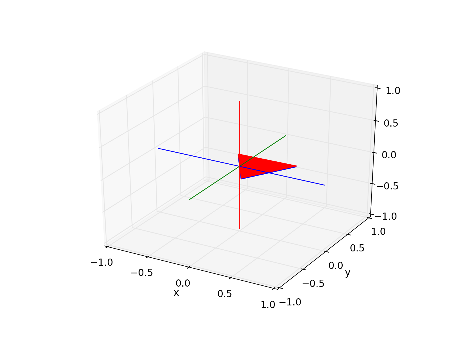
orientation : Visualization of 3D orientations as animated triangle.
- Orientation_OGLMuch faster 3D orientation viewer, based
on OpenGL
1-dimensional and 3-dimensional data can be viewed. It also allows to inspect the variables of the current workspace.
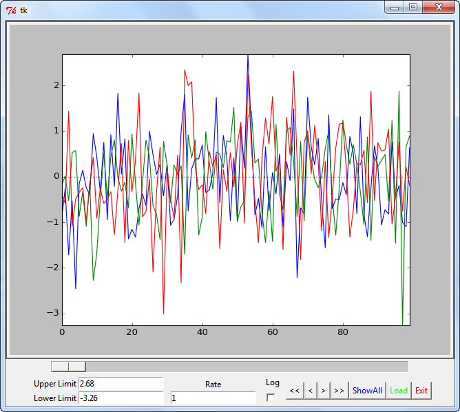
Interactively analyze time-series data …
Functions
view.ts()… Viewer for time-series data

Improved viewability of 3D data.
view.orientation()… Visualize and animate orientations, expressed as quaternions.
Class
|
Orientation viewer utilizing OpenGL |
Details
- This module includes two functions:
An interactive viewer for time-series data (“view.ts”)
An animation of 3D orientations, expressed as quaternions (“view.orientation”)
- For the time-series viewer, variable types that can in principle be plotted are:
np.ndarray
pd.core.frame.DataFrame
pd.core.series.Series
Viewer can be used to inspect a single variable, or to select one from the current workspace.
- Notable aspects:
Based on Tkinter, to ensure that it runs on all Python installations.
Resizable window.
Keyboard-based interaction.
Logging of marked events.
- view.orientation(quats, out_file=None, title_text=None, deltaT=100)[source]
Calculates the orienation of an arrow-patch used to visualize a quaternion. Uses “_update_func” for the display.
- Parameters:
quats (array [(N,3) or (N,4)]) – Quaterions describing the orientation.
out_file (string) – Path- and file-name of the animated out-file (“.mp4”). [Default=None]
title_text (string) – Name of title of animation [Default=None]
deltaT (int) – interval between frames [msec]. Smaller numbers make faster animations.
Example
To visualize a rotation about the (vertical) z-axis:
>>> # Set the parameters
>>> omega = np.r_[0, 10, 10]     # [deg/s]
>>> duration = 2
>>> rate = 100
>>> q0 = [1, 0, 0, 0]
>>> out_file = 'demo_patch.mp4'
>>> title_text = 'Rotation Demo'
>>>
>>> # Calculate the orientation
>>> num_rep = duration*rate
>>> omegas = np.tile(omega, [num_rep, 1])
>>> q = skin.quat.calc_quat(omegas, q0, rate, 'sf')
>>>
>>> orientation(q, out_file, 'Well done!', deltaT=1000./rate)
Note
Seems to be slow. So unless you need a movie, better use “Orientation_OGL”.
- view.ts(data=None)[source]
Show the given time-series data. In addition to the (obvious) GUI-interactions, the following options are available:
- Keyboard interaction:
f … forward (+ 1/2 frame)
n … next (+ 1 frame)
b … back ( -1/2 frame)
p … previous (-1 frame)
z … zoom (x-frame = 10% of total length)
a … all (adjust x- and y-limits)
x … exit
- Optimized y-scale:
Often one wants to see data symmetrically about the zero-axis. To facilitate this display, adjusting the “Upper Limit” automatically sets the lower limit to the corresponding negative value.
- Logging:
When “Log” is activated, right-mouse clicks are indicated with vertical bars, and the corresponding x-values are stored into the users home-directory, in the file “[varName].log”. Since the name of the first value is unknown the first events are stored into “data.log”.
- Load:
Pushing the “Load”-button shows you all the plottable variables in your namespace. Plottable variables are:
ndarrays
Pandas DataFrames
Pandas Series
Examples
To view a single plottable variable:
>>> x = np.random.randn(100,3)
>>> view.ts(x)
To select a plottable variable from the workspace
>>> x = np.random.randn(100,3)
>>> t = np.arange(0,10,0.1)
>>> y = np.sin(x)
>>> view.ts(locals)