
Distribution of a Sample Mean
One sample t-test for a mean value
To check the mean value of normally distributed data against a reference value, we typically use the one sample t-test, which is based on the t-distribution.
If we knew the mean and the standard deviation of a normally distributed population, we would know exactly the standard error, and use values from the normal distribution to determine how likely it is to find a certain mean value, given the population mean and standard deviation. However, in practice we have to estimate the mean and standard deviation from the sample, and the resulting distribution for the mean value deviates slightly from a normal distribution.
Let us look at a specific example: we take 100 normally distributed data, with a mean of 7 and with a standard deviation of 3. What is the chance of finding a mean value at a distance of 0.5 or more from the mean?
Answer: The probability from the t-test is 0.0006, and from the normal distribution 0.0004 (see attached .py and .ipynb-file)
Example
Let us look at a specific example: we take 100 normally distributed data, with a mean of 7 and with a standard deviation of 3. What is the chance of finding a mean value at a distance of 0.5 or more from the mean? Answer: The probability from the t-test in the example is 0.057, and from the normal distribution 0.054
Since it is very important to understand the basic principles of how we arrive at the t-statistic and the corresponding p-value for this test, let me illustrate the underlying statistics by going step-by-step through the analysis:

Left: Frequency histogram of the sample data, together with a normal fit. The sample mean, which is very close to the population mean, is indicated with a yellow triangle; the value to be checked with a red triangle. Right: t-distribution for n-1 degrees of freedom. At the bottom the normalized value of sample mean (yellow triangle) and value to be checked (red triangle). The red shaded area corresponds to the p-value.
- We have a population, with a mean value of 7 and a standard deviation of 3.
- From that population an observer takes 100 random samples. The sample mean is 7.10, close to but different from the real mean. The sample standard deviation is 3.12, and the standard error of the mean 0.312. This gives the observer an idea about the variability of the population.
- The observer knows that the distribution of the real mean follows a t-distribution, and that the standard error of the mean characterizes the width of that distribution.
- How likely it is that the real mean has a value of \(x_0\) (e.g. 6.5, indicated by the red triangle in the Figure above, left)? To find that out, this value has to be transformed, by subtracting the sample mean, and dividing by the standard error. (Figure above, right). This provides the t-statistic for this test (-1.93).
- The corresponding p-value, which tells us how likely it is that the real mean has a value of 6 or more extreme relative to the sample mean, is given by the red shaded area under the curve-wings: 2*CDF(t-statistic)=0.057, which means that the difference to 6.5 is just not significant. (The factor “2” comes from the fact that we have to check in both tails.)
Wilcoxon signed rank sum test
If our data are not normally distributed, we cannot use the t-test (although this test is fairly robust against deviations from normality). Instead, we must use a non-parametric test on the mean value. We can do this by performing a Wilcoxon signed rank sum test.
(The following description and example has been taken from Altman, Table 9.2)
This method has three steps:
- Calculate the difference between each observation and the value of interest.
- Ignoring the signs of the differences, rank them in order of magnitude.
- Calculate the sum of the ranks of all the negative (or positive) ranks, corresponding to the observations below (or above) the chosen hypothetical value.
In the Table below you see an example, where the significance to a deviation from the value of 7725 is tested. The rank sum of the negative values gives \(3+5=8\), and can be looked up in the corresponding tables to be significant. In practice, your computer program will nowadays do this for you. This example also shows another feature of rank evaluations: tied values (here \(7515\)) get accorded their mean rank (here \(1.5\)).
| Subject | Daily energy intake (kJ) | Difference from 7725 kJ | Ranks of differences |
|---|---|---|---|
| 1 | 5260 | 2465 | 11 |
| 2 | 5470 | 2255 | 10 |
| 3 | 5640 | 2085 | 9 |
| 4 | 6180 | 1545 | 8 |
| 5 | 6390 | 1335 | 7 |
| 6 | 6515 | 1210 | 6 |
| 7 | 6805 | 920 | 4 |
| 8 | 7515 | 210 | 1.5 |
| 9 | 7515 | 210 | 1.5 |
| 10 | 8230 | -505 | 3 |
| 11 | 8770 | -1045 | 5 |

Comparison of Two Groups
Paired T-Test
When you compare two groups with each other, we have to distinguish between two cases. In the first case, we compare two values recorded from the same subject at two specific times. For example, we measure the size of students when they enter primary school and after their first year, and check if they have been growing. Since we are only interested in the difference between the first and the second measurement, this test is called paired t-test, and is essentially equivalent to a one-sample t-test for the mean difference.
Unpaired T-Test
The second test is if we compare two independent groups. For example, we can compare the effect of a two medications given to two different groups of patients, and compare how the two groups respond. This is called an unpaired t-test, or t-test for two independent groups.
If we have two independent samples the variance of the difference between their means is the sum of the separate variances, so the standard error of the difference in means is the square root of the sum of the separate variances:
where \(\bar{x}_i\) is the mean of the i-th sample, and se indicates the standard error.
Non-parametric Comparison of Two Groups: Mann-Whitney Test
If the measurement values from the two groups are not normally distributed we have to resort to a non-parametric test. The most common test for that is the Mann-Whitney(-Wilcoxon) test. Watch out, because this test is sometimes also referred to as Wilcoxon rank-sum test. This is different from the Wilcoxon signed rank sum test!
Statistical Tests vs Statistical Modeling
With the advent of cheap computing power, statistical modeling has been a booming field. This has also affected classical statistical analysis, as most problems can be viewed from two perspectives: you can either make a statistical hypothesis, and verify or falsify that hypothesis; or you can make a statistical model, and analyse the significance of the model parameters.
Let me use a classical t-test as an example.
Classical t-test
Let us take performance measurements from a racing team, on two different occasions. During Race_1, the members of the team achieve a score of [ 79., 100., 93., 75., 84., 107., 66., 86., 103., 81., 83., 89., 105., 84., 86., 86., 112., 112., 100., 94.], and during Race_2 [ 92., 100., 76., 97., 72., 79., 94., 71., 84., 76., 82., 57., 67., 78., 94., 83., 85., 92., 76., 88.].
These numbers can be generated, and a t-test comparing the two groups can be done, with the following Python commands:
from scipy import stats
random.seed(123)
race_1 = np.round(randn(20)*10+90)
race_2 = np.round(randn(20)*10+85)
(t, pVal) = stats.ttest_rel (race_1, race_2)
print('The probability that the two distributions are equal is {0}'.format(pVal))
The command random.seed(123) initializes the random number generator with the number \(123\), which ensures that two consecutive runs of this code produce the same result, corresponding to the numbers given above.
Statistical Modeling
import pandas as pd
import statsmodels.formula.api as sm
np.random.seed(123)
df = pd.DataFrame({'Race1': race_1, 'Race2':race_2})
result = sm.ols(formula='I(Race2-Race1) ~ 1', data=df).fit()
print(result.summary())
The important line is the last but one, which produces the \(results\). Thereby the ordinary least square (ols) function from statsmodels tests the model which describes the difference between the results of Race1 and those of Race2 with only an offset (also called intercept in the language of modeling). In other words, our model has only one paramter, the intercept. The results below show that the probability that this intercept is 0 is only 0.03: the difference is significant.
                             OLS Regression Results
==============================================================================
Dep. Variable:       I(Race2 - Race1)   R-squared:                       0.000
Model:                            OLS   Adj. R-squared:                  0.000
Method:                 Least Squares   F-statistic:                       nan
Date:                Sun, 08 Feb 2015   Prob (F-statistic):                nan
Time:                        18:48:06   Log-Likelihood:                -85.296
No. Observations:                  20   AIC:                             172.6
Df Residuals:                      19   BIC:                             173.6
Df Model:                           0
Covariance Type:            nonrobust
==============================================================================
                 coef    std err          t      P>|t|      [95.0% Conf. Int.]
------------------------------------------------------------------------------
Intercept     -9.1000      3.950     -2.304      0.033       -17.367    -0.833
==============================================================================
Omnibus:                        0.894   Durbin-Watson:                   2.009
Prob(Omnibus):                  0.639   Jarque-Bera (JB):                0.793
Skew:                           0.428   Prob(JB):                        0.673
Kurtosis:                       2.532   Cond. No.                         1.00
==============================================================================
The output is explained in more model in the chapter [chapter:Models]. The important point here is that the t- and p-value for the intercept are the same as with the classical t-test above.
Comparison of More Groups
Analysis of Variance
The idea behind the ANalysis Of VAriance (ANOVA) is to divide the variance into the variance between groups, and that within groups, and see if those distributions match the null hypothesis that all groups come from the same distribution. The variables that distinguish the different groups are often called factors.
(By comparison, t-tests look at the mean values of two groups, and check if those are consistent with the assumption that the two groups come from the same distribution.)
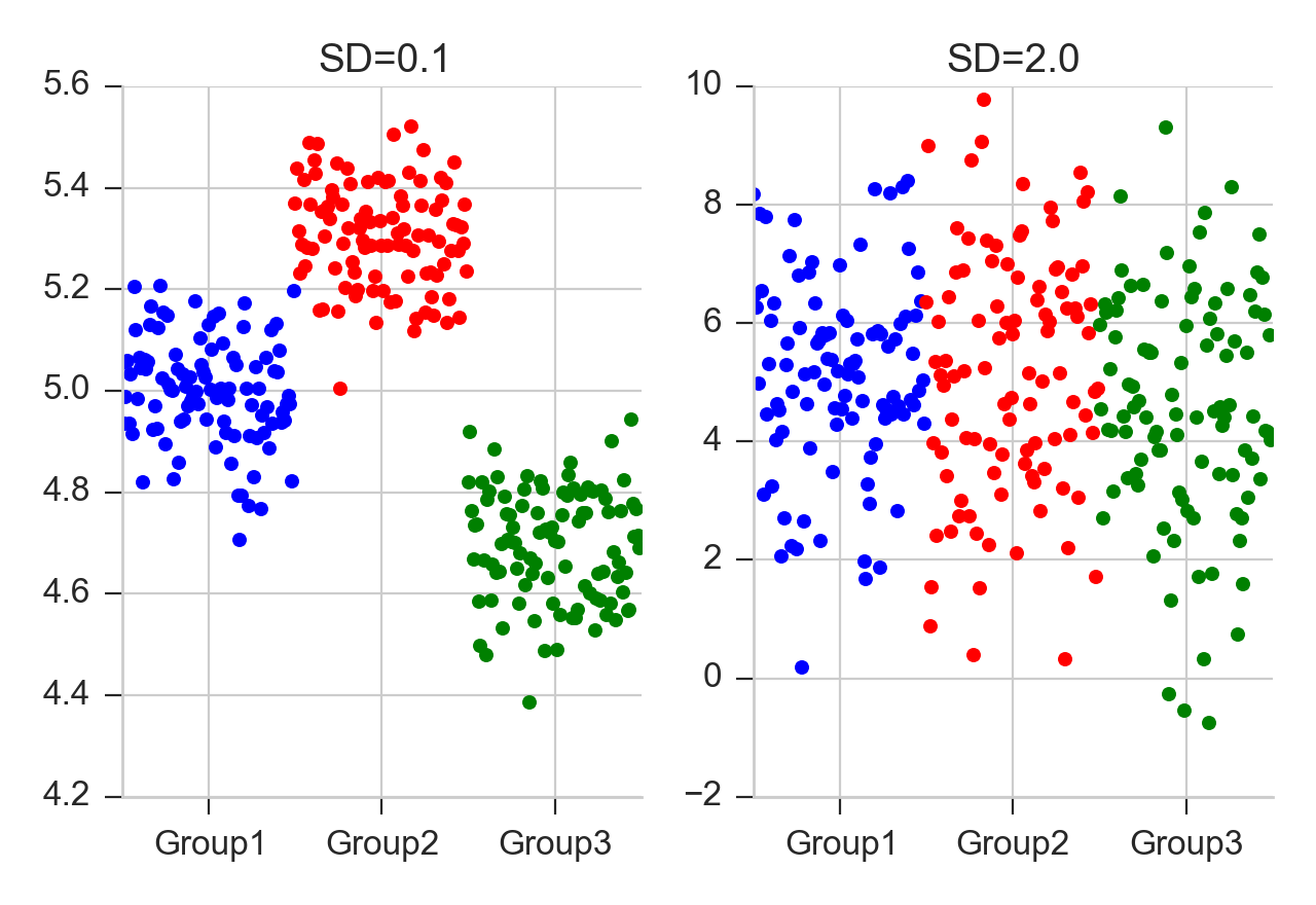
In both cases, the difference between the two groups is the same. But left, he difference within the groups is smaller than the differences between the groups, whereas right, the difference within the groups is larger than the difference between.
For example, if we compare a group with No treatment, another with treatment A, and a third with treatment B, then we perform a one factor ANOVA, sometimes also called one-way ANOVA, with “treatment” the one analysis factor. If we do the same test with men and with women, then we have a two-factor or two-way ANOVA, with “gender” and “treatment” as the two treatment factors. Note that with ANOVAs, it is quite important to have exactly the same number of samples in each analysis group!
Because the null hypothesis is that there is no difference between the groups, the test is based on a comparison of the observed variation between the groups (i.e. between their means) with that expected from the observed variability between subjects. The comparison takes the general form of an F test to compare variances, but for two groups the t test leads to exactly the same answer.

The long blue line indicates the grand mean over all data. The SS_{Error} describes the variability “within”the groups, and the SS_{Treatment}`(summed over all respective points!) the variability “between” groups.
The one-way ANOVA assumes all the samples are drawn from normally distributed populations with equal variance. To test this assumption, you can use the Levene test.
ANOVA uses traditional standardized terminology. The definitional equation of sample variance is \(s^2=\textstyle\frac{1}{n-1}\sum(y_i-\bar{y})^2\), where the divisor is called the degrees of freedom (DF), the summation is called the sum of squares (SS), the result is called the mean square (MS) and the squared terms are deviations from the sample mean. ANOVA estimates 3 sample variances: a total variance based on all the observation deviations from the grand mean, an error variance based on all the observation deviations from their appropriate treatment means and a treatment variance. The treatment variance is based on the deviations of treatment means from the grand mean, the result being multiplied by the number of observations in each treatment to account for the difference between the variance of observations and the variance of means. If the null hypothesis is true, all three variance estimates are equal (within sampling error).
The fundamental technique is a partitioning of the total sum of squares SS into components related to the effects used in the model. For example, the model for a simplified ANOVA with one type of treatment at different levels.
The number of degrees of freedom DF can be partitioned in a similar way: one of these components (that for error) specifies a chi-squared distribution which describes the associated sum of squares, while the same is true for “treatments” if there is no treatment effect.
Example: one-way ANOVA
As an example, let us take the red cell folate levels (\(\mu g/l\)) in three groups of cardiac bypass patients given different levels of nitrous oxide ventilation (Amess et al, 1978), described in the Python code example below. I first show the result of this ANOVA test, and then explain the steps to get there.
              DF     SS       MS       F   p(>F)
C(treatment)   2  15515.76  7757.88  3.71  0.043
Residual      19  39716.09  2090.32   NaN    NaN
- First the “Sums of squares (SS)” are calculated. Here the SS between treatments is 15515.88, and the SS of the residuals is 39716.09 . The total SS is the sum of these two values.
- The mean squares (“MS”) is the SS divided by the corresponding degrees of freedom (“df”).
- The F-test or variance ratio test is used for comparing the factors of the total deviation. The F-value is the larger mean squares value divided by the smaller value. (If we only have two groups, the F-value is the square of the corresponding t-value. See listing below.)
- Under the null hypothesis that two normally distributed populations have equal variances we expect the ratio of the two sample variances to have an F Distribution. From the F-value, we can look up the corresponding p-value.
Multiple Comparisons
The Null hypothesis in a one-way ANOVA is that the means of all the samples are the same. So if a one-way ANOVA yields a significant result, we only know that they are not the same.
However, often we are not just interested in the joint hypothesis if all samples are the same, but we would also like to know for which pairs of samples the hypothesis of equal values is rejected. In this case we conduct several tests at the same time, one test for each pair of samples. (Typically, this is done with t-tests)
This results, as a consequence, in a multiple testing problem: since we perform multiple comparison tests, we should compensate for the risk of getting a significant result, even if our null hypothesis is true. This can be cone by correcting the p-values to account for this. We have a number of options to do so:
- Tukey HSD
- Bonferroni correction
- Holms correction
- ... and others ...
Tukey’s Test
Tukey’s test, sometimes also referred to as the Tukey Honest Significant Difference (HSD) method, controls for the Type I error rate across multiple comparisons and is generally considered an acceptable technique. It is based on a formula very similar to that of the t-test. In fact, Tukey’s test is essentially a t-test, except that it corrects for multiple comparisons.
The formula for Tukey’s test is:
where \(Y_A\) is the larger of the two means being compared, \(Y_B\) is the smaller of the two means being compared, and \(SE\) is the standard error of the data in question. This \(q_s\) value can then be compared to a q value from the studentized range distribution, which takes into account the multiple comparisons. If the qs value is larger than the critical value obtained from the distribution, the two means are said to be significantly different. Note that the studentized range statistic is the same as the t-statistic except for a scaling factor (np.sqrt(2)).
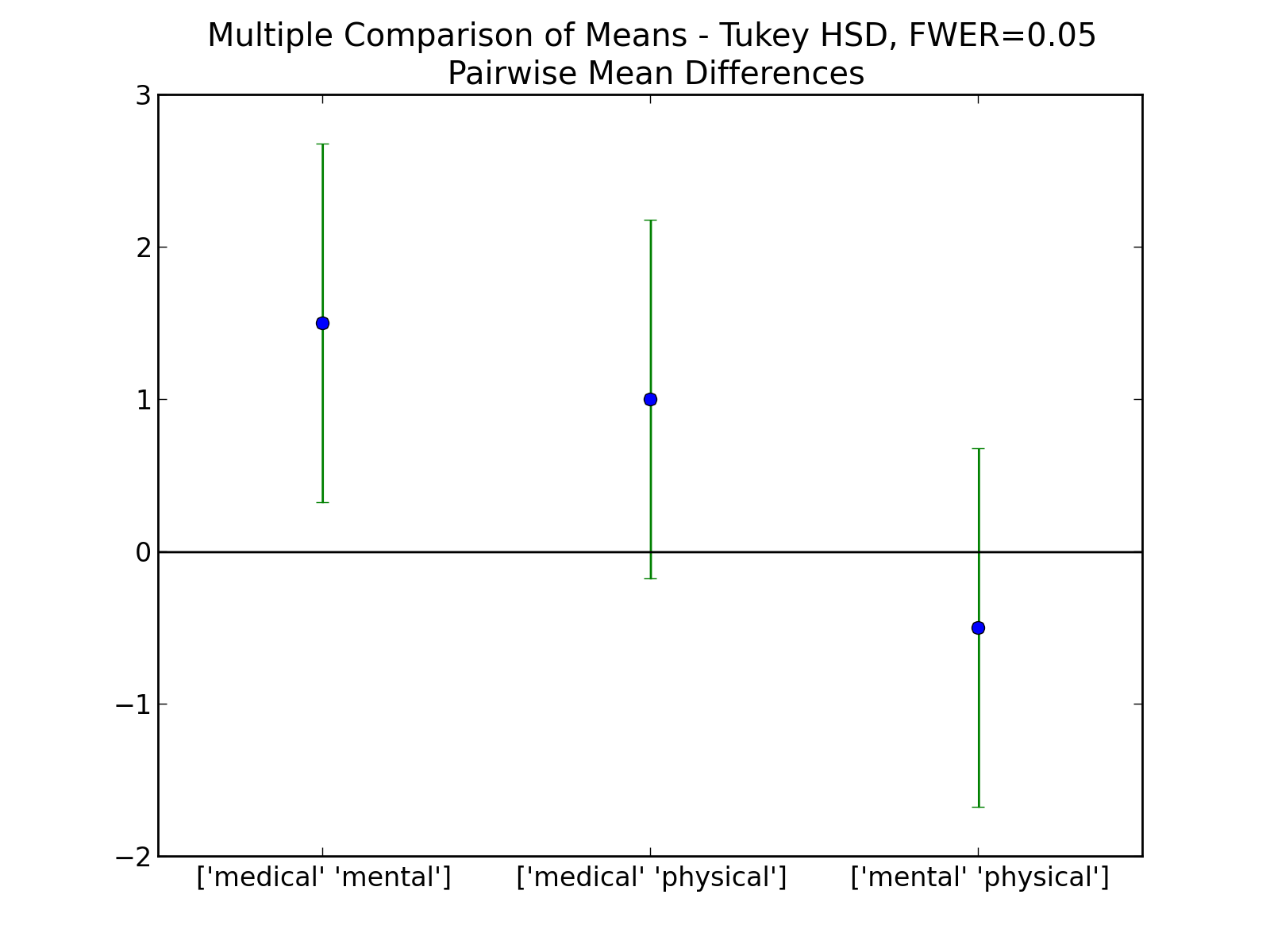
Comparing the means of multiple groups - here three different treatment options.
Bonferroni correction
Tukey’s studentized range test (HSD) is a test specific to the comparison of all pairs of k independent samples. Instead we can run t-tests on all pairs, calculate the p-values and apply one of the p-value corrections for multiple testing problems. The simplest - and at the same time quite conservative - approach is to divide the required p-value by the number of tests that we do (Bonferroni correction). For example, if you perform 4 comparisons, you check for significance not at p=0.05, but at p=0.0125.
While multiple testing is not yet included in Python standardly, you can get a number of multiple-testing corrections done with the statsmodels package:
In[7]: from statsmodels.sandbox.stats.multicomp import multipletests
In[8]: multipletests([.05, 0.3, 0.01], method='bonferroni')
Out[8]:
(array([False, False,  True], dtype=bool),
array([ 0.15,  0.9 ,  0.03]),
0.016952427508441503,
0.016666666666666666)
Holms correction
The Holm adjustment sequentially compares the lowest p-value with a Type I error rate that is reduced for each consecutive test. For example, if you have three groups (and thus three comparisons), this means that the first p-value is tested at the .05/3 level (.017), the second at the .05/2 level (.025), and third at the .05/1 level (.05). This method is generally considered superior to the Bonferroni adjustment.
Kruskal-Wallis test
When we compare two groups to each other, we use the t-test when the data are normally distributed and the non-parametric Mann-Whitney test otherwise. For three or more groups, the test for normally distributed data is the ANOVA-test; for not-normally distributed data, the corresponding test is the Kruskal-Wallis test. When the null hypothesis is true the test statistic for the Kruskal-Wallis test follows the Chi squared distribution.
Exercises
One or Two Groups
Paired T-test and Wilcoxon signed rank sum test
The daily energy intake from 11 healthy women is [5260., 5470., 5640., 6180., 6390., 6515., 6805., 7515., 7515., 8230., 8770.] kJ.
- Is this value significantly different from the recommended value of 7725?
(Correct answer: yes, p_ttest=0.018, p_Wilcoxon=0.026)
t-test of independent samples
In a clinic, 15 lazy patients weight [76., 101., 66., 72., 88., 82., 79., 73., 76., 85., 75., 64., 76., 81., 86.] kg, and 15 sporty patients weigh [ 64., 65., 56., 62., 59., 76., 66., 82., 91., 57., 92., 80., 82., 67., 54.] kg.
- Are the lazy patients significantly heavier?
(Correct answer: yes, p=0.045)
Normality test
- Are the two datasets normally distributed?
(Correct answer: yes, they are)
Mann-Whitney test
- Are the lazy patients still heavier, if you check with the Mann-Whitney test?
(Correct answer: yes, p=0.039)
Multiple Groups
(The following example is taken from the really good, but somewhat advanced book by AJ Dobson: “An Introduction to Generalized Linear Models”)
Get the data
The file https://github.com/thomas-haslwanter/statsintro/blob/master/Data/data_others/Table 6.6 Plant experiment.xls contains data from an experiment with plants in three different growing conditions. Get the data into Python. Hint: use the module xlrd
Perform an ANOVA
- Are the three groups different?
(Correct answer: yes, they are.)
Multiple Comparisons
- Using the Tukey test, which of the pairs are different?
(Correct answer: only TreamtmentA and TreatmentB differ)
Kruskal-Wallis
- Would a non-parametric comparison lead to a different result?
(Correct answer: no)