Characterizing a Distribution

Population and samples

While the whole population of a group has certain characteristics, we can typically never measure all of them. In many cases, the population distribution is described by an idealized, continuous distribution function.

In the analysis of measured data, in contrast, we have to confine ourselves to investigate a (hopefully representative) sample of this group, and estimate the properties of the population from this sample.

Continuous Distribution Functions

A continuous distribution function describes the distribution of a population, and can be represented in several equivalent ways:

Probability Density Function (PDF)

The PDF, or density of a continuous random variable, is a function that describes the relative likelihood for a random variable \(X\) to take on a given value \(x\). In the mathematical fields of probability and statistics, a random variate x is a particular outcome of a random variable X: the random variates which are other outcomes of the same random variable might have different values.

Since the likelihood to find any given value cannot be less than zero, and since the variable has to have some value, the PDF has the following properties:

• \(PDF(x) \geq 0\,\forall \,x \in \mathbb{R}\)
• \(\int\limits_{ - \infty }^\infty {PDF(x)dx = 1}\)

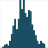
Probability Density Function (PDF) of a value x. The integral over the PDF between a and b gives the likelihood of finding the value of x in that range.

Cumulative Distribution Function (CDF)

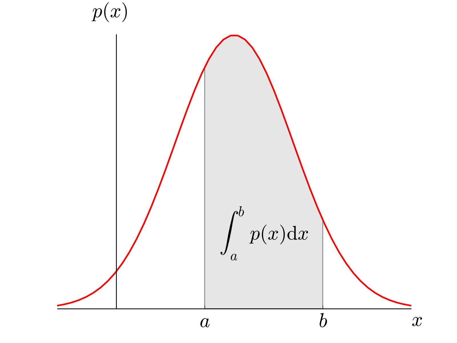
The probability to find a value between \(a\) and \(b\) is given by the integral over the PDF in that range (see Fig. [fig:PDF]), and the Cumulative Distribution Function tells you for each value which percentage of the data has a lower value (see Figure below). Together, this gives us

\[\mathbb{P}(a \leq X \leq b) = \int\limits_a^b {PDF(x)dx} = CDF(b) - CDF(a)\]

Probability Density Function (left) and Cumulative distribution function (right) of a normal distribution.

Other important presentations of Probability Densities

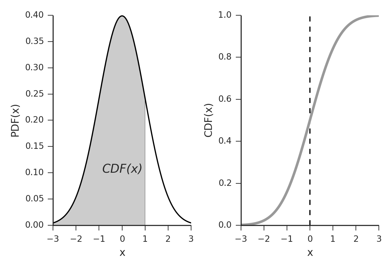
The Figure Utility functions for continuous distributions, here for the normal distribution. shows a number of functions are commonly used to select appropriate points a distribution function:

• Probability density function (PDF): note that to obtain the probability for the variable appearing in a certain interval, you have to integrate the PDF over that range.

  Example: What is the chance that a man is between 160 and 165 cm tall?

• Cumulative distribution function (CDF): gives the probability of obtaining a value smaller than the given value.

  Example: What is the chance that a man is less than 165 cm tall?

• Survival function (SF): 1-CDF: gives the probability of obtaining a value larger than the given value. It can also be interpreted as the proportion of data “surviving” above a certain value.

  Example: What is the chance that a man is larger than 165 cm?

• Percentile point function (PPF): the inverse of the CDF. Answers the question “Given a certain probability, what is the corresponding value for the CDF?”

  Example: Given that I am looking for a man who is smaller than 95% of all other men, what size does the subject have to be?

• Inverse survival function (ISF): the name says it all.

  Example: Given that I am looking for a man who is larger than 95% of all other men, what size does the subject have to be?

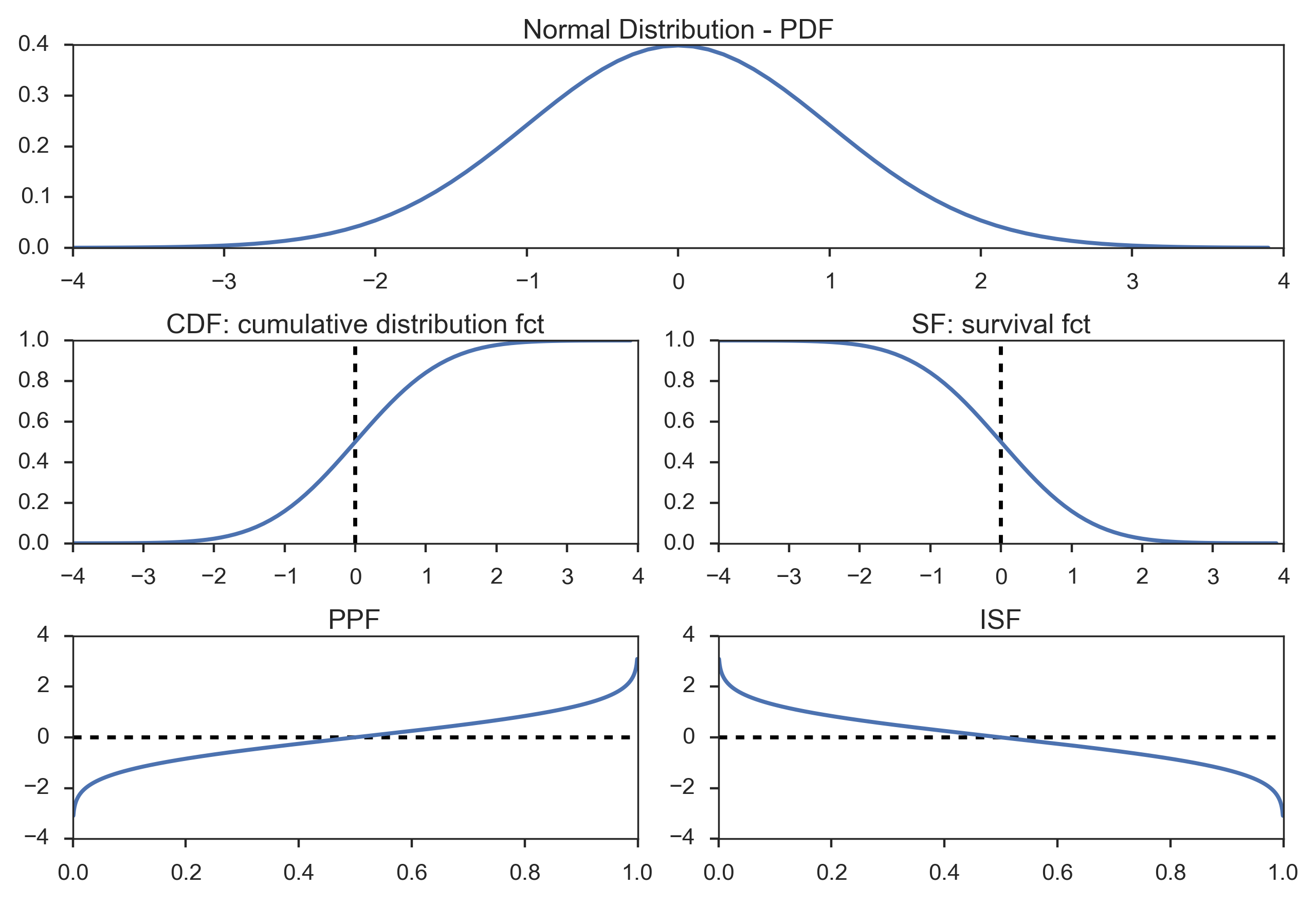
Utility functions for continuous distributions, here for the normal distribution.

Note:

In Python, the most elegant way of working with distribution function is a two-step procedure:

• In the first step, you create your distribution (e.g. nd = stats.norm()). Note that is a distribution (in Python parlance a “frozen distribution”), not a function yet!
• In the second step, you decide which function you want to use from this distribution, , and calculate the function value for the desired x-input (e.g. y = nd.cdf(x))

Distribution Center

When we have a datasample from a distribution, we can characterize the center of the distribution with different parameters:

Mean

By default, when we talk about the mean value we mean the arithmetic mean \(\bar{x}\):

\[\bar{x} = \frac{{\sum\limits_{i = 1}^n {{x_i}} }}{n}\]

Median

The median is that value that comes half-way when the data are ranked in order. In contrast to the mean, it is not affected by outlying data points.

Mode

The mode value is the most frequently occurring value in a distribution.

Geometric Mean

In some situations the geometric mean can be useful to describe the location of a distribution. It is usually close to the median, and can be calculated via the arithmetic mean of the log of the values.

Quantifying Variability

Range

This one is fairly easy: it is the difference between the highest and the lowest data value. The only thing that you have to watch out for: after you have acquired your data, you have to check for outliers, i.e. data points with a value much higher or lower than the rest of the data. Often, such points are caused by errors in the selection of the sample or in the measurement procedure. There are a number of tests to check for outliers. One of them is to check for data which lie more than 1.5*inter-quartile-range (IQR) above or below the first/third quartile (see below).

Percentiles

The Cumulative distribution function (CDF) tells you for each value which percentage of the data has a lower value (Figure Utility functions for continuous distributions, here for the normal distribution.). The value below which a given percentage of the values occur is called centile or percentile, and corresponds to a value with a specified cumulative frequency.

For example, when you look for the data range which includes 95% of the data, you have to find the \(2.5^{th}\) and the \(97.5^{th}\) percentile of your sample distribution.

The \(50^{th}\) percentile is the median.

Also important are the quartiles, i.e. the \(25^{th}\) and the \(75^{th}\) percentile. The difference between them is sometimes referred to as inter-quartile range (IQR).

Median, upper and lower quartile are used for the data display in box plots.

Standard Deviation and Variance

The variance (SD) of a distribution is defined as

\[var = \frac{{\sum\limits_{i = 1}^n {({x_i-\bar{x}})^2} }}{n-1}\]

Note that we divide by n-1 rather than the more obvious n: dividing by \(n\) gives the variance of the observations around the sample mean, but we virtually always consider our data as a sample from some larger population and wish to use the sample data to estimate the variability in the population. Dividing by \(n-1\) gives us a better estimate of the population variance.

The Figure below indicates why the sample standard deviation underestimates the standard deviation of the underlying distribution.

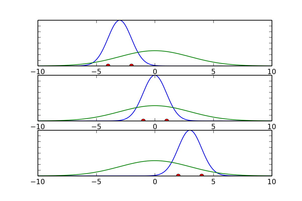
Gaussian distributions fitted to selections of data from the underlying distribution: While the average mean of a number of samples converges to the real mean, the sample standard deviation underestimates the standard deviation from the distribution.

Since the t-distribution has longer tails than the normal distribution, it is much less sensitive to outliers (see Figure above).

The standard deviation is simply given by the square root of the variance:

\[s = \sqrt{var}\]

In statistics it is often common to denote the population standard deviation with \(\sigma\), and the sample standard deviation with \(s\).

Watch out: in Python, by default the variance is calculated for “n”. You have to set “ddof=1” to obtain the variance for “n-1”:

In[19]: data = arange(7,14)

In[20]: std(data, ddof=0)
Out[20]: 2.0

In[21]: std(data, ddof=1)
Out[21]: 2.1602468994692865

Standard Error

While the standard deviation is a good measure for the distribution of your values, often you are more interested in the distribution of the mean value. For example, when you measure the response to a new medication, you might be interested in how well you can characterize this response, i.e. is how well you know the mean value. This measure is called the standard error of the mean, or sometimes just the standard error. In a single sample from a population with a standard deviation of \(\sigma\) the variance of the sampling distribution of the mean is \(\sigma^2/n\), and so the standard error of the mean is \(\sigma/\sqrt{n}\).

For the sample standard error of the mean, which is the one you will be working with most of the time, we have

\[SE = \frac{s}{\sqrt{n}} = \sqrt{\frac{{\sum\limits_{i = 1}^n {({x_i-\bar{x}})^2} }}{n-1}} \cdot \frac{1}{\sqrt{n}}\]

Confidence Intervals

The most informative parameter that you can give for a statistical variable is arguably its confidence interval. The confidence interval reports the range that contains the true value for your parameter with a likelihood of \(\alpha\)%.

Most of the time you want to determine the confidence interval for normally distributed data, which is given by

\[ci = mean \pm std * N_{ISF}(\alpha)\]

where \(std\) is the standard deviation, and \(N_{ISF}(\alpha)\) the inverse survival function for the normal distribution. For the 95% two-sided confidence intervals, for example, you have to set \(\alpha=0.025\) and \(\alpha=0.975\) .

Note: If you want to know the confidence interval for the mean value, you have to replace the standard deviation by the standard error!

Parameters Describing the Form of a Distribution

In scipy.stats, continuous distribution functions are characterized by their location and their scale. Should the definition of a distribution require more than two parameters, the following parameters are called shape parameters. The exact meaning of each parameter can be found in the function definition.

For example, for the normal distribution, (location/shape) are given by (mean/standard deviation) of the distribution. In contrast, for the uniform distribution, location/shape are given by the (start/end) of the range where the distribution is different from zero.

Location

A location parameter x_0 determines the “location” or shift of a distribution.

\[f_{x0}(x)=f(x-x_0)\]

Examples of location parameters include the mean, the median, and the mode.

Scale

The scale parameter describes the width of a probability distribution. If s is large, then the distribution will be more spread out; if s is small then it will be more concentrated. If the probability density exists for all values of s, then the density (as a function of the scale parameter only) satisfies

\[f_s(x) = f(x/s)/s,\]

where f is the density of a standardized version of the density.

Shape Parameters

A shape parameter is any parameter of a probability distribution that is neither a location parameter nor a scale parameter. If location and shape already completely determine the distribution (as is the case for e.g. the normal distribution or the exponential distribution, etc.), then these distributions don’t have any shape parameter. It follows that the skewness and kurtosis of these distribution are constants.

Skewness

Distributions are skewed if they depart from symmetry. For example, if you have a measurement that cannot be negative, which is usually the case, then we can infer that the data have a skewed distribution if the standard deviation is more than half the mean. Such an asymmetry is referred to as positive skewness. The opposite, negative skewness, is rare.

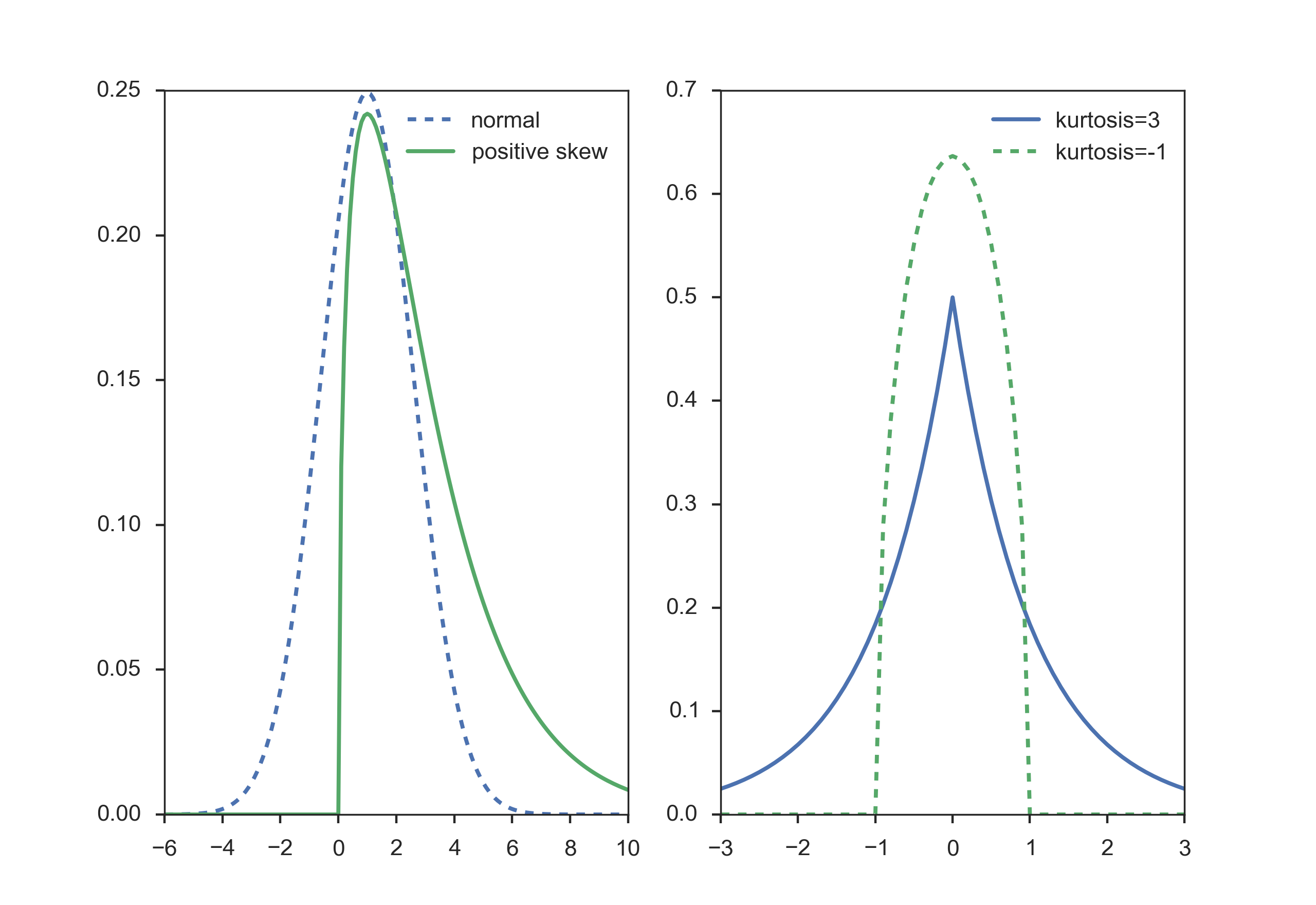
{Left) Normal distribution, and distribution with positive skewness. Right) The (leptokurtic) Laplace distribution has an excess kurtosis of 3, and the (platykurtic) Wigner semicircle distribution an excess kurtosis of -1.}

Kurtosis

Kurtosis is any measure of the “peakedness” of the probability distribution. Distributions with negative or positive excess kurtosis are called platykurtic distributions or leptokurtic distributions respectively.

Distribution Functions

The variable for a standardized distribution function is often called statistic. So you often find expressions like “the z-statistic” (for the normal distribution function), the “t-statistic” (for the t-distribution) or the “F-statistic” (for the F-distribution).

Normal Distribution

The Normal distribution or Gaussian distribution is by far the most important of all the distribution functions. This is due to the fact that the mean values of all distribution functions approximate a normal distribution for large enough sample numbers. Mathematically, the normal distribution is characterized by a mean value \(\mu\), and a standard deviation \(\sigma\):

\[\label{eq_normal} f_{\mu,\sigma} (x) = \frac{1}{\sigma \sqrt{2 \pi}} e^{-( x - \mu )^2 /2 \sigma^2}\]

where \(-\infty<x<\infty\), and \(f_{\mu,\sigma}\) is the probability density function (PDF) .

Normal Distribution

For smaller sample numbers, the sample distribution can show quite a bit of variability. For example, look at 25 distributions generated by sampling 100 numbers from a normal distribution:

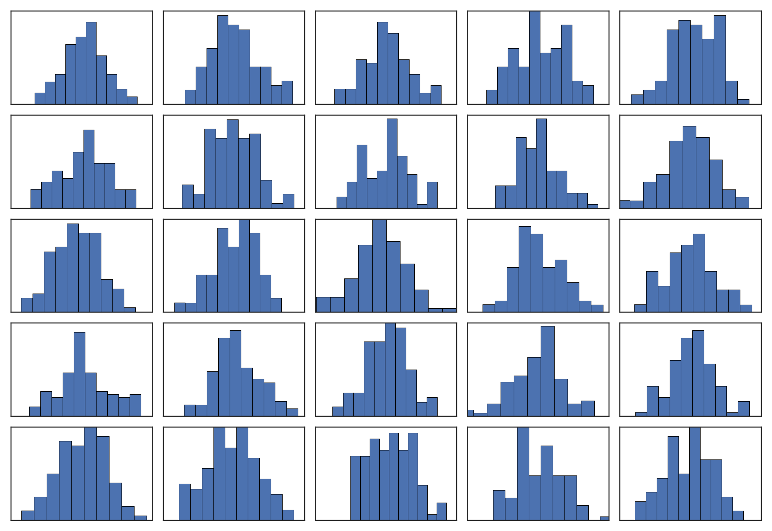
25 randomly generated normal distributions of 100 points.

Some examples of applications are:

• If the average man is 175 cm tall with a standard deviation of 6 cm, what is the probability that a man found at random will be 183 cm tall?
• If the average man is 175 cm tall with a standard deviation of 6 cm and the average woman is 168 cm tall with a standard deviation of 3 cm, what is the probability that the average man from a given sample will be shorter than the average woman from a given sample?
• If cans are assumed to have a standard deviation of 4 grams, what does the average weight need to be in order to ensure that the 99% of all cans have a weight of at least 250 grams?

The normal distribution with parameters \(\mu\) and \(\sigma\) is denoted as \(N(\mu,\sigma)\). If the random variate (rv) X is normally distributed with expectation \(\mu\) and standard deviation \(\sigma\), one denotes: \(\,X \sim N(\mu,\sigma)\) or \(\,X \in N(\mu,\sigma)\).

30_figs_DistributionNormal.ipynb

Area under +/- 1, 2, and 3 standard deviations of a normal distribution.

Range	Prob. of being within	Prob. of being outside
mean \(\pm\) 1SD	0.683	0.317
mean \(\pm\) 2SD	0.954	0.046
mean \(\pm\) 3SD	0.9973	0.0027

Since a very frequent computational steps is the calculation of the intervals containing 95% of the data, I give an explicit code example of that step:

In [33]:  from scipy import stats
In [34]:  mu = -2
In [35]:  sigma = sqrt(0.5)
In [36]:  myDistribution = stats.norm(mu, sigma)
In [37]:  significanceLevel = 0.05
In [38]:  myDistribution.ppf([significanceLevel/2, 1-significanceLevel/2])
Out[38]:  array([-3.38590382, -0.61409618]

Example of how to calculate the interval of the PDF containing 95% of the data, for the green curve in the Figure above.

Central Limit Theorem

The central limit theorem states that for identically distributed independent random variables (also referred to as random variates), the mean of a sufficiently large number of these variables will be approximately normally distributed.

The figure below shows that averaging over 10 uniformly distributed data already produces a smooth, almost Gaussian distribution.

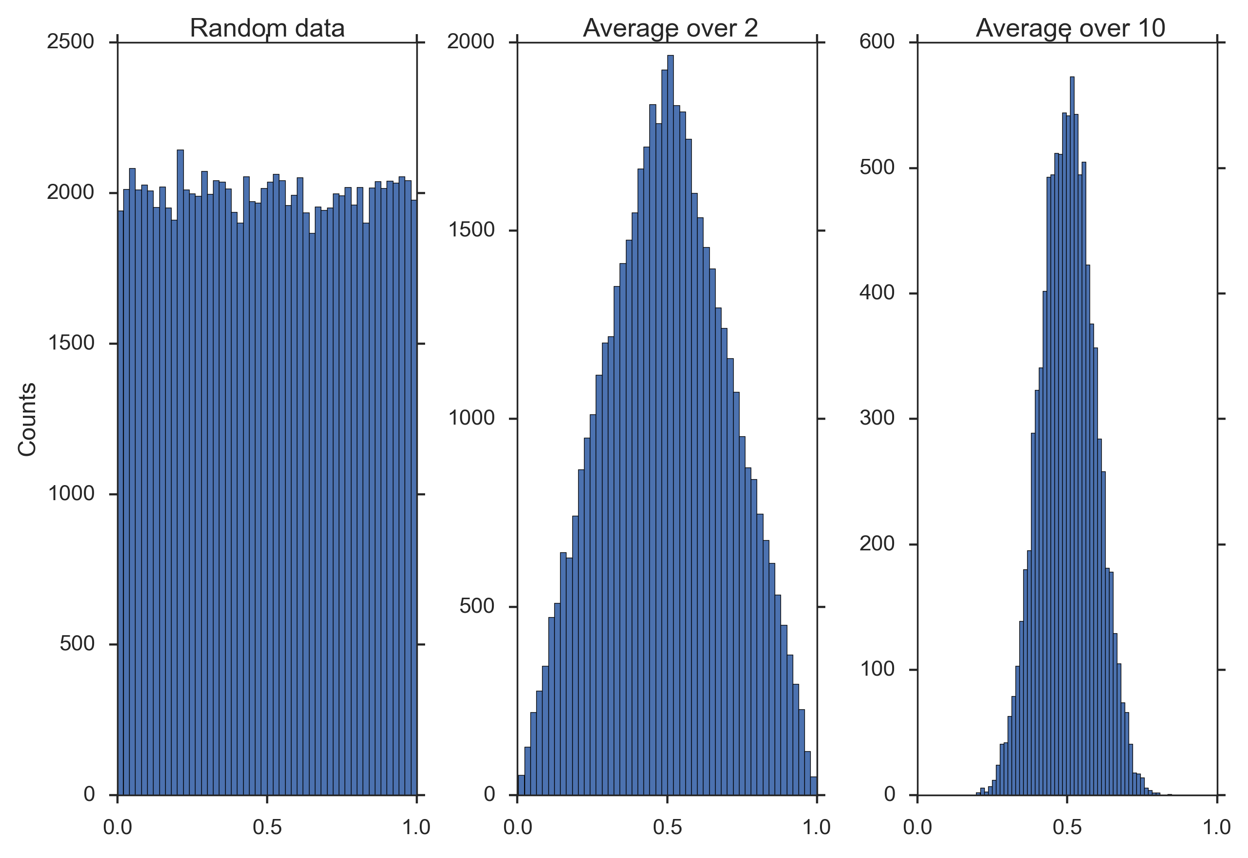
Demonstration of the “Central Limit Theorem”: Left) Histogram of random data between 0 and 1. Center) Histogram of average over two datapoints.) Right) Histogram of average over 10 datapoints.

'''
Practical demonstration of the central limit theorem

'''

# author: Thomas Haslwanter, date: July-2014

# Import standard packages
import numpy as np
import matplotlib.pyplot as plt
import seaborn as sns
import os

# additional packages
import mystyle

sns.set(context='poster', style='ticks')

def main():
    '''Demonstrate central limit theorem.'''
    # Generate data
    ndata = 1e5
    nbins = 50
    data = np.random.random(ndata)
    
    # Show them
    fig, axs = plt.subplots(1,3)
    #mystyle.set(14)
    #sns.set_context('paper')
    #sns.set_style('whitegrid')
    
    axs[0].hist(data,bins=nbins)
    axs[0].set_title('Random data')
    axs[0].set_xticks([0, 0.5, 1])
    axs[0].set_ylabel('Counts')
    
    axs[1].hist( np.mean(data.reshape((ndata/2,2)),  axis=1), bins=nbins)
    axs[1].set_xticks([0, 0.5, 1])
    axs[1].set_title(' Average over 2')
    
    axs[2].hist( np.mean(data.reshape((ndata/10,10)),axis=1), bins=nbins)
    axs[2].set_xticks([0, 0.5, 1])
    axs[2].set_title(' Average over 10')
    
    plt.tight_layout()
    mystyle.printout_plain('CentralLimitTheorem.png')
    
    plt.show()    
    
if __name__ == '__main__':
   main() 

Application Example

To illustrate the ideas behind the use of distribution functions, let us go step-by-step through the analysis of the following problem:

The average weight of a newborn child in the US is 3.5 kg, with a standard deviation of 0.76 kg. If we want to check all children that are significantly different from the typical baby, what should we do with a child that is born with a weight of 2.6 kg?

• Find the distribution that characterizes healthy babies.
• Calculate the CDF at the interesting value (CDF(2.6 kg) = 0.118).
• Interpret the result (“If the baby is healthy, the chance that its weight deviates by at least the observed value from the mean is 2*11.8% = 23.6% - This is not significant”).

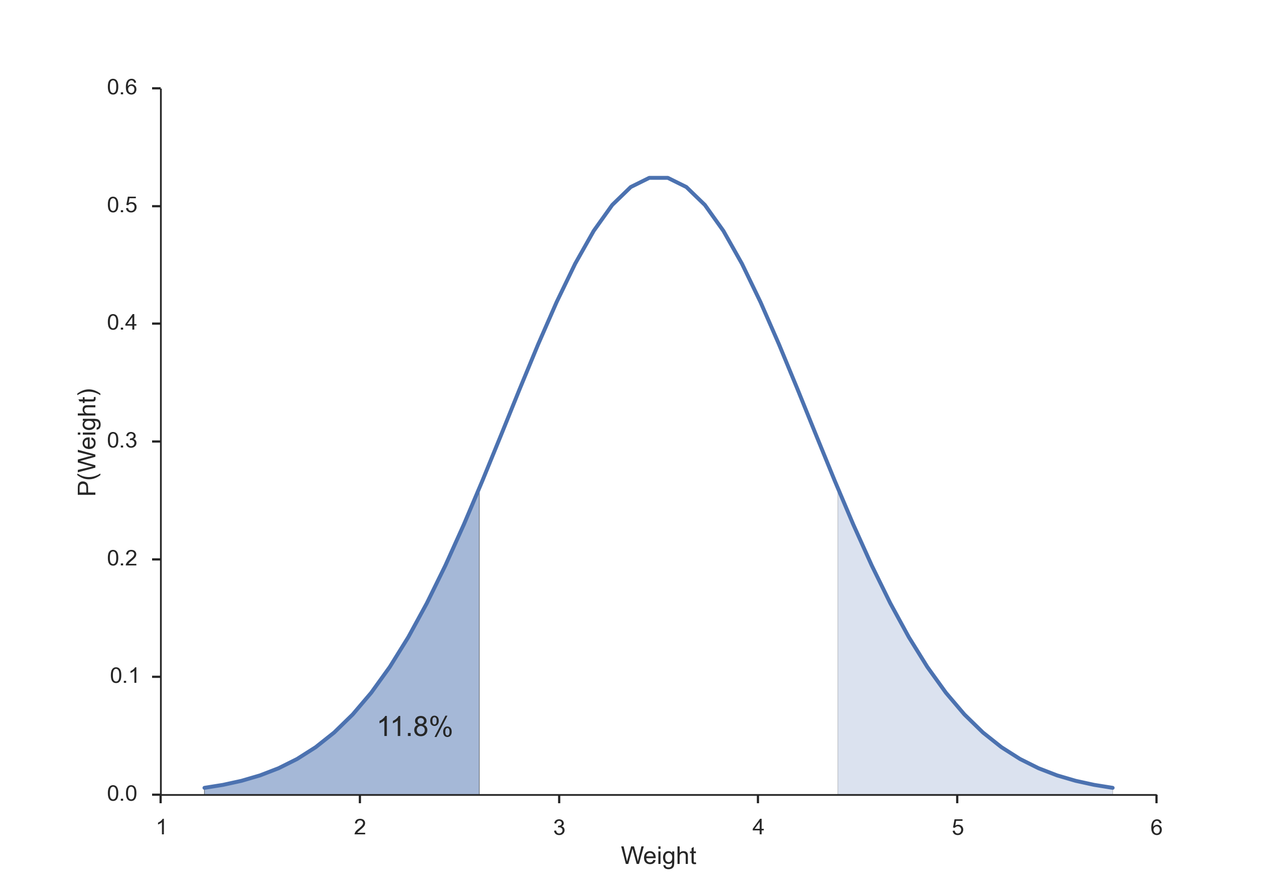
The chance that a healthy baby weighs 2.6 kg or less is 11.8% (darker blue area). The chance that the difference from the mean is that much is twice that much, as the lighter blue area must be added.

Other Continuous Distributions

The distributions you will encounter most frequently are:

• Normal distribution - the “ideal” continuous probability distribution
• t-distribution - for sample distributions (What you will probably use most often.)
• Chi-square distribution - for describing variability
• F-distribution - for comparing variability

In the following, we will describe these distributions in more detail. Other distributions you should have heard about will be mentioned briefly:

• Lognormal distribution - a normal distribution, plotted on an exponential scale. Often used to convert a strongly skewed distribution into a normal one.
• Weibull distribution - mainly used for reliability or survival data.
• Exponential distribution - exponential curves
• uniform distribution - when everything is equally likely.

t Distribution

For a small number of samples (ca <10) from a normal distribution, the distribution of the mean deviates slightly from the normal distribution. The reason is that the sample mean does not coincide exactly with the population mean. This modified distribution is the t-distribution, and converges for larger values towards the normal distribution.

The t-distribution was first described by a researcher working under the pseudonym of “Student”, and the corresponding test is therefore sometimes referred to as Student’s t-test.

If \(\bar{x}\) is the sample mean, and s the sample standard deviation, then

\[t = \frac{\bar{x}-\mu}{s/ \sqrt{n}}\]

A very frequent application of the t-distribution is in the calculation of Confidence intervals:

\[ci = mean \pm std * t_{df,\alpha}\]

In [27]: n = 20
In [28]: df = n-1
In [29]: alpha = 0.05
In [30]: stats.t(df).ppf(1-alpha/2)
Out[30]: 2.093

In [31]: stats.norm.ppf(1-alpha/2)
Out[31]: 1.960

Calculating the t-values for confidence intervals, for n = 20 and :math:`alpha=0.05`. For comparison, I also calculate the corresponding value from the normal distribution.

In Python, the 95% confidence interval for the mean can be obtained with a one-liner:

alpha = 0.95
df = len(data)-1
ci = stats.t.interval(alpha, df, loc=mean(data), scale=stats.sem(data))

t Distribution

Since the t-distribution has longer tails than the normal distribution, it is much less sensitive to outliers (see Figure below).

The t-distribution is much more robust against outliers than the normal distribution.

Chi-square Distribution

The Chi-square distribution is related to normal distribution in a simple way: If a random variable \(X\) has a normal distribution (\(X \in N(0,1)\)), then \(X^2\) has a chi-square distribution, with one degree of freedom (\(X^2 \in \chi_{1}^2\)). The sum squares of \(n\) independent and standard normal random variables has a chi-square distribution with \(n\) degrees of freedom:

\[\sum\limits_{i = 1}^n {X_i^2} \in \chi_{n}^2\]

Chi-square Distribution

Application Example

A pill producer is ordered to deliver pills with a standard deviation of \(\sigma=0.05\). From the next batch of pills you pick \(n=13\) random samples. These samples \(x_1, x_2, . . . , x_n\) have a weight of 3.04, 2.94, 3.01, 3.00, 2.94, 2.91, 3.02, 3.04, 3.09, 2.95, 2.99, 3.10, 3.02 g.

Question: is the standard deviation larger than allowed?

Answer:

Since the Chi-square distribution describes the distribution of the summed squares of random variates from a standard normal distribution, we have to normalize our data before we calculate the corresponding CDF-value:

\[1 - CD{F_{{\chi ^2}_{(n - 1)}}}\left( {\sum {(\frac{{x - \bar x}}{\sigma }} {)^2}} \right) = 0.1929\]

Interpretation: if the batch of pills is from a distribution with a standard deviation of \(\sigma=0.05\), the likelihood of obtaining a chi-square value as large or larger than the one observed is about 19%, so it is not atypical. In other words, the batch matches the expected standard deviation.

F Distribution

Named after Sir Ronald Fisher, who developed the F distribution for use in determining critical values in ANOVAs (ANalysis Of VAriance). The cutoff values in an F table are found using three variables:

• ANOVA numerator degrees of freedom
• ANOVA denominator degrees of freedom
• significance level

ANOVA compares the size of the variance between two different samples. This is done by dividing the larger variance over the smaller variance. The formula for the resulting F statistic is:

\[F(r_1, r_2) = \frac{\chi_{r1} ^2 /r_1}{\chi_{r2} ^2 /r_2}\]

where \(\chi_{r1}^2\) and \(\chi_{r2}^2\) are the chi-square statistics of sample one and two respectively, and \(r_1\) and \(r_2\) are their degrees of freedom, i.e. the number of observations.

F-Test of Equality of Variances

If you want to investigate whether two groups have the same variance, you have to calculate the ratio of the sample standard deviations squared:

\[F = \frac{S_x^2}{S_y^2}\]

where \(S_x\) ist he sample standard deviation of the first sample, and \(S_y\) the sample standard deviation for the second sample.

Application Example

Take for example the case that you want to compare two methods to measure eye movements. The two methods can have different accuracy and different precision. With your test you want to determine if the precision of the two methods is equivalent, or if one method is more precise than the other.

Accuracy and precision of a measurement are two different characteristics!

When you look 20 deg to the right, you get the following results: Method 1: [20.7, 20.3, 20.3, 20.3, 20.7, 19.9, 19.9, 19.9, 20.3, 20.3, 19.7, 20.3] Method 2: [ 19.7, 19.4, 20.1, 18.6, 18.8, 20.2, 18.7, 19. ]

The F statistic is \(F = 0.494\), and has \(n-1\) and \(m-1\) degrees of freedom, where \(n\) and \(m\) are the number of recordings with each method. The code sample below shows that the F statistic is close to the center of the distribution, so we cannot reject the hypothesis that the two methods have the same precision.

In [1]:  method1 = array([20.7,  20.3,  20.3,  20.3,  20.7,  19.9,  19.9,  19.9,  20.3,
      20.3,  19.7,  20.3])
In [2]:  method2 = array([ 19.7,  19.4,  20.1,  18.6,  18.8,  20.2,  18.7,  19. ])
In [3]:  fval = var(method1, ddof=1)/var(method2, ddof=1)
In [4]:  fd = stats.f(len(method2)-1,len(method2)-1)
In [5]:  p = fd.cdf(fval)
In [6]:  print p
Out[6]:  0.041
In [7]:  if (p<0.025) or (p>0.975):
            print 'There is a significant difference between the two distributions.'

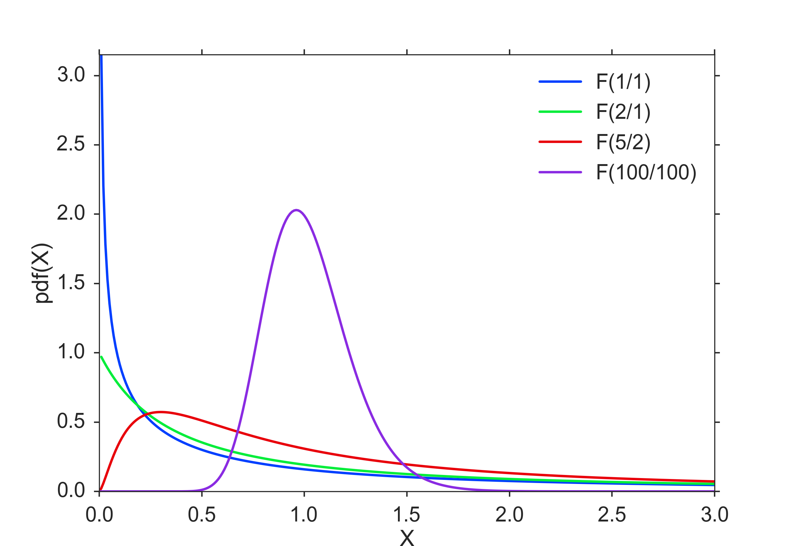
F Distribution

Lognormal Distribution

In some circumstances a set of data with a positively skewed distribution can be transformed into a symmetric distribution by taking logarithms. Taking logs of data with a skewed distribution will often give a distribution that is near to normal (see Figure below).

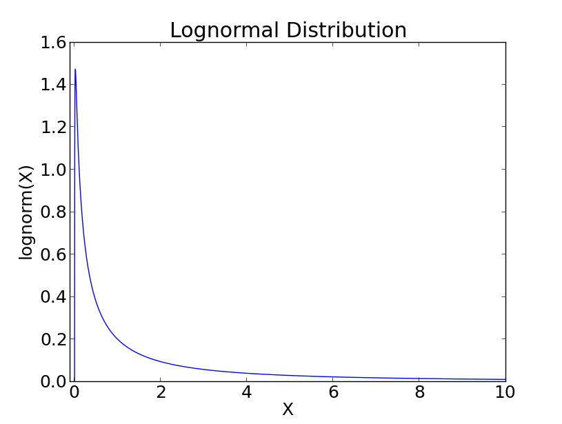
Plotted against a linear abscissa.

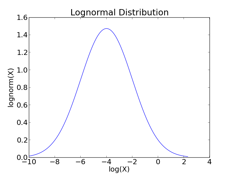
Plotted against a logarithmic abscissa. Plotted against a logarithmic abscissa.

Weibull Distribution

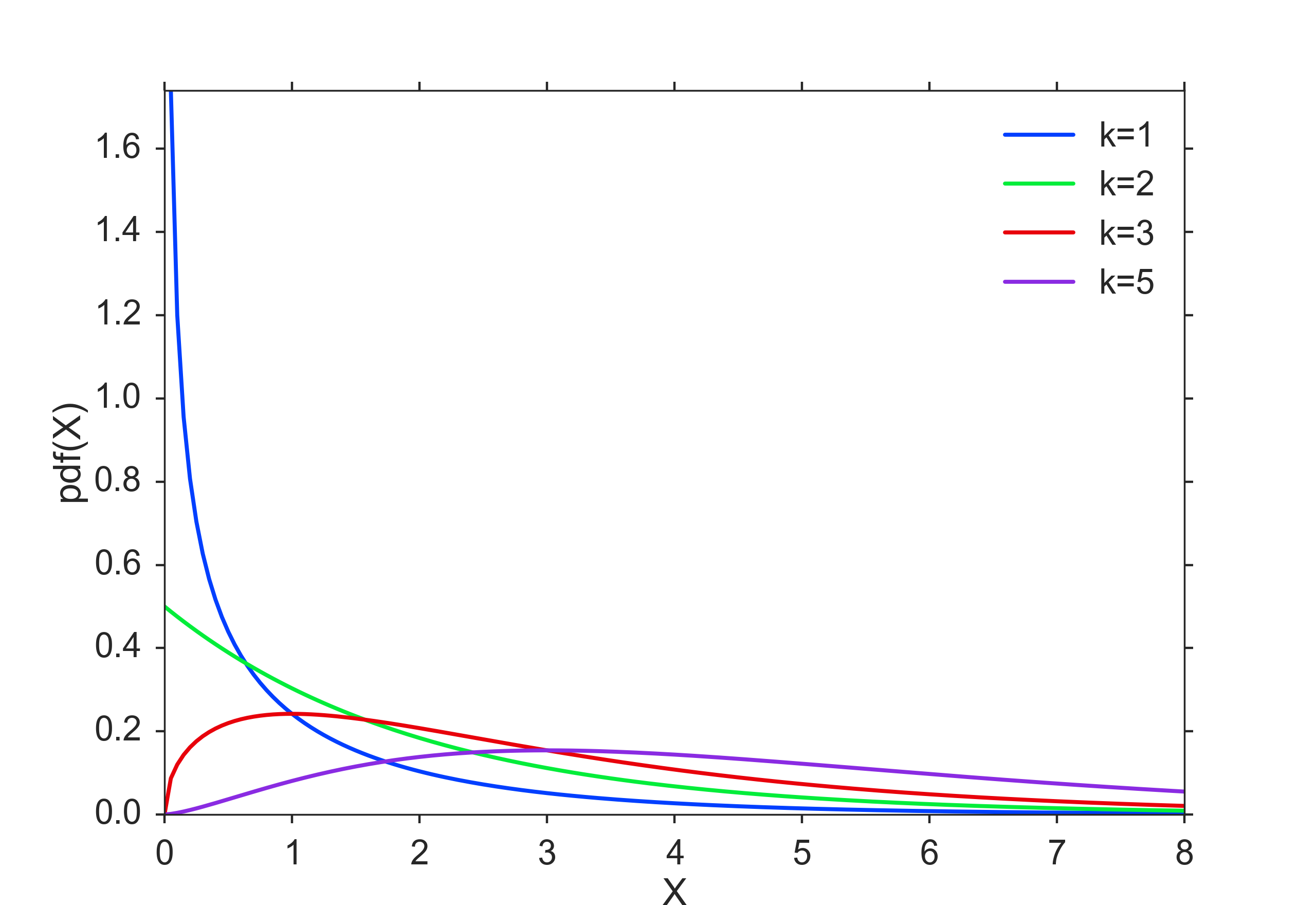
The Weibull distribution is the most commonly used distribution for modeling reliability data or “survival” data. It has two parameters, which allow it to handle increasing, decreasing or constant failure-rates (see Figure below). It is defined as

\[\begin{split} \label{eq_weibull} f_x (x) = \begin{cases} k \frac{x^{k-1}}{\lambda^k} e^{-(x/\lambda)^{k}} & x\geq0 \\ 0 & x<0 , \end{cases}\end{split}\]

where k > 0 is the shape parameter and \(\lambda > 0\) is the scale parameter of the distribution. Its complementary cumulative distribution function is a stretched exponential function.

If the quantity x is a “time-to-failure”, the Weibull distribution gives a distribution for which the failure rate is proportional to a power of time. The shape parameter, k, is that power plus one, and so this parameter can be interpreted directly as follows:

• A value of k < 1 indicates that the failure rate decreases over time. This happens if there is significant “infant mortality”, or defective items failing early and the failure rate decreasing over time as the defective items are weeded out of the population.
• A value of k = 1 indicates that the failure rate is constant over time. This might suggest random external events are causing mortality, or failure.
• A value of k > 1 indicates that the failure rate increases with time. This happens if there is an “aging” process, or parts that are more likely to fail as time goes on.

In the field of materials science, the shape parameter k of a distribution of strengths is known as the Weibull modulus.

Weibull Distribution

Exponential Distribution

For a stochastic variable X with an exponential distribution, the probability distribution function is:

\[\begin{split}\label{eq_exponential} f_x (x) = \begin{cases} \lambda e^{- \lambda x}, & \mbox{if } x \ge 0 \\ 0, & \mbox{if } x < 0 \end{cases}\end{split}\]

The exponential PDF is shown in the figure below

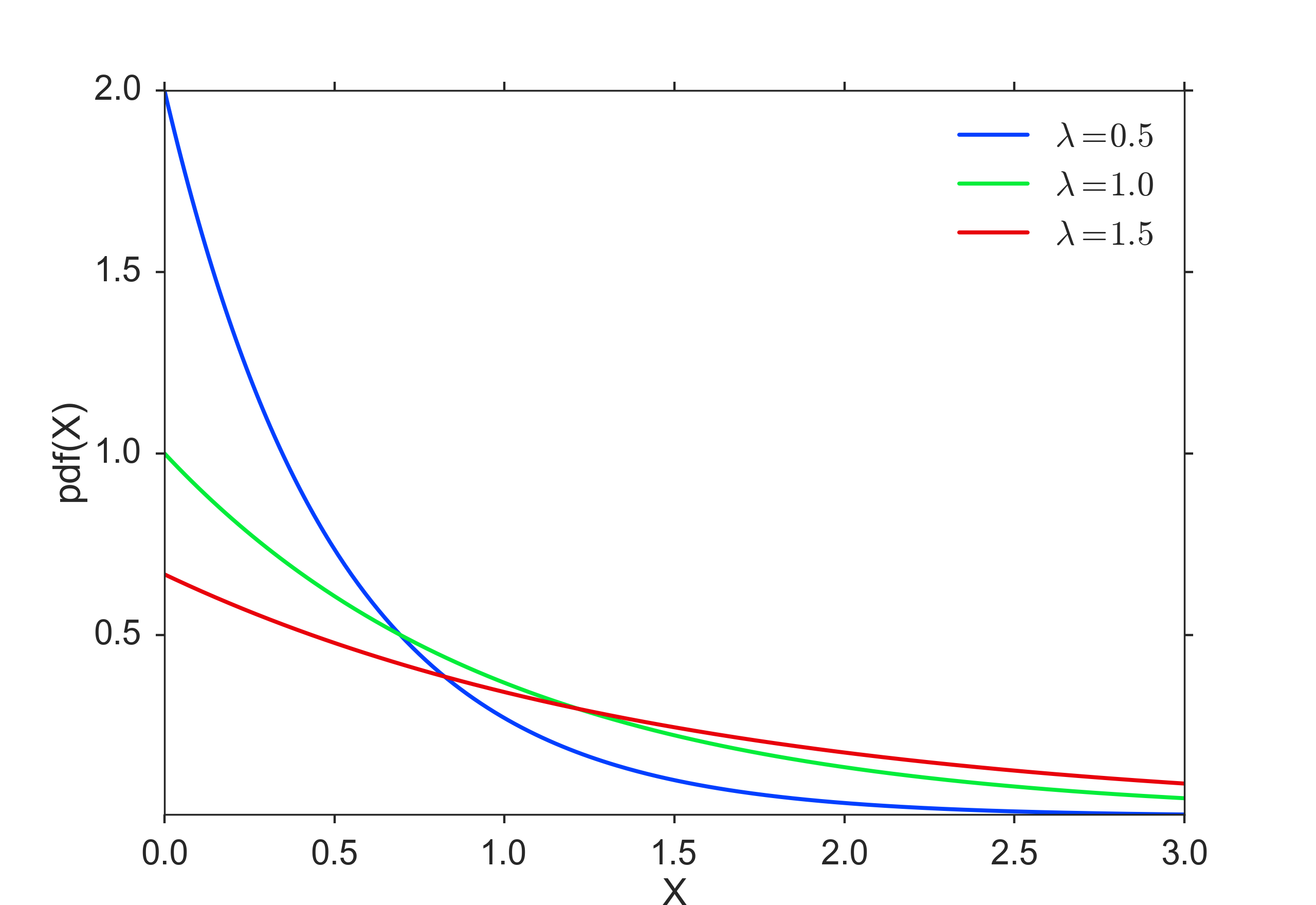
Exponential Distribution

Uniform Distribution

This is a simple one: an even probability for all data values (see Figure below). Not very common for real data.

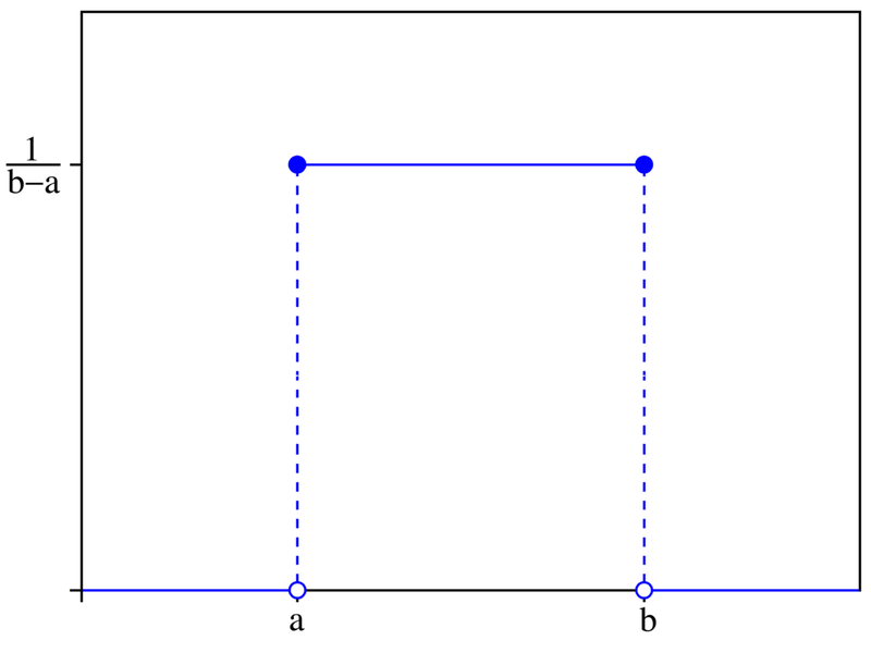
Uniform Distribution

Programs: Continuous Distribution Functions

Working with distribution functions in Python takes a bit to get used to. But once you get the concept, it is marvellously easy. In my opinion, the most logical way is first to define the function, with all the parameters that it requires; and then, to use the methods of this function, e.g. PDF or CDF:

In [1]: from scipy import stats
In [2]: myDF = stats.norm(5,3)
In [3]: x = linspace(-5, 15, 101)
In [4]: y = myDF.pdf(x)

31_figs_DistContinuous.ipynb

Discrete Distributions

While the functions describing continuous distributions are referred to as probability distribution functions, discrete distributions are described by probability mass functions.

Two discretely distributions are commonly encountered: the binomial distribution, and the Poisson distribution. These two have the following properties:

	Mean	Variance
Binomial	\(n \cdot p\)	\(np(1-p)\)
Poisson	\(\lambda\)	\(\lambda\)

Table: Properties of discrete distributions.

The big difference between those two functions that you have to keep in mind: applications of the Binomial function have an inherent upper limit (e.g. when you throw dice five times, each side can come up a maximum of five times); in contrast, the Poisson distribution does not have an inherent upper limit (e.g. how many people you know).

Binomial Distribution

The Binomial is associated with the question “Out of a given number of trials, how many will succeed?” Some example questions that are modeled with a Binomial distribution are:

• Out of ten tosses, how many times will this coin land ”heads”?
• From the children born in a given hospital on a given day, how many of them will be girls?
• How many students in a given classroom will have green eyes?
• How many mosquitos, out of a swarm, will die when sprayed with insecticide?

We conduct \(n\) repeated experiments where the probability of success is given by the parameter \(p\) and add up the number of successes. This number of successes is represented by the random variable \(X\). The value of \(X\) is then between 0 and \(n\).

When a random variable X has a Binomial Distribution with parameters \(p\) and \(n\) we write it as \(\,X \sim Bin(n,p)\) or \(\,X \sim B(n,p)\) and the probability mass function is given at \(X=k\) by the equation:

\[\begin{split}P\left[X = k\right] = \begin{cases} {n \choose k} p^k \left(1-p\right)^{n-k}\ & 0 \le k \le n \\ 0 & \mbox{otherwise} \end{cases} \quad 0 \leq p \leq 1, \quad n \in \mathbb{N}\end{split}\]

where \({n \choose k}={n! \over k!(n-k)!}\)

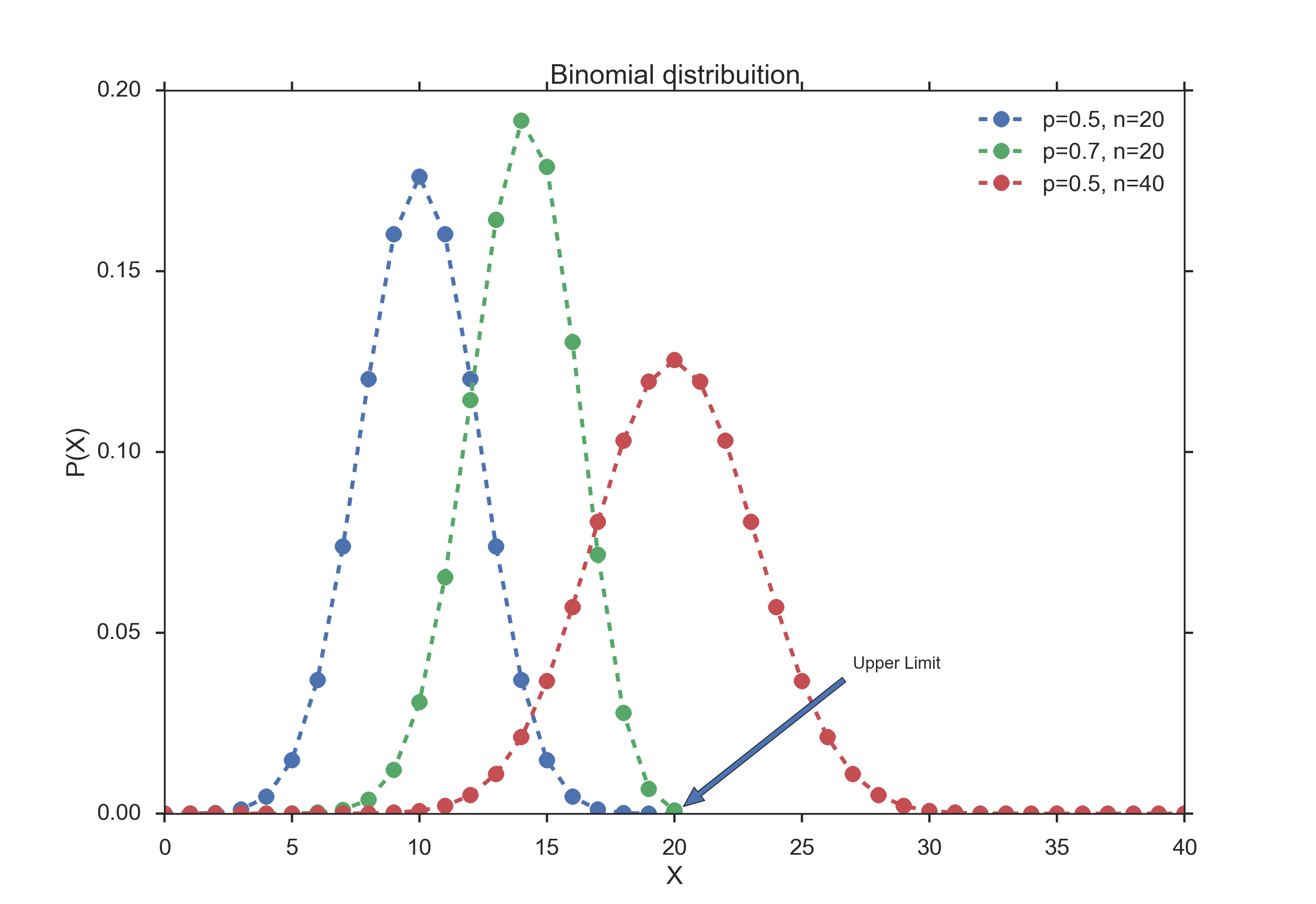
Binomial Distribution

The binomial distribution for n = 1 is sometimes referred to as Bernoulli Distribution.

For n trials, we have the following properties:

• mean: np
• variance: n p (1-p)

Poisson Distribution

Any French speaker will notice that “Poisson” means “fish”, but really there’s nothing fishy about this distribution. It’s actually pretty straightforward. The name comes from the mathematician Siméon-Denis Poisson (1781-1840).

The Poisson Distribution is very similar to the Binomial Distribution. We are examining the number of times an event happens. The difference is subtle. Whereas the Binomial Distribution looks at how many times we register a success over a fixed total number of trials, the Poisson Distribution measures how many times a discrete event occurs, over a period of continuous space or time. There isn’t a “total” value n. As with the previous sections, let’s examine a couple of experiments or questions that might have an underlying Poisson nature.

• How many pennies will I encounter on my walk home?
• How many children will be delivered at the hospital today?
• How many products will I sell after airing a new television commercial?
• How many mosquito bites did you get today after having sprayed with insecticide?
• How many defects will there be per 100 metres of rope sold?

What’s a little different about this distribution is that the random variable \(X\) which counts the number of events can take on any non-negative integer value. In other words, I could walk home and find no pennies on the street. I could also find one penny. It’s also possible (although unlikely, short of an armored-car exploding nearby) that I would find 10 or 100 or 10,000 pennies.

Instead of having a parameter p that represents a component probability like in the Binomial distribution, this time we have the parameter “lambda” or \(\lambda\) which represents the “average or expected” number of events to happen within our experiment. The probability mass function of the Poisson is given by

\[P(X=k)=\frac{e^{-\lambda}\lambda^k}{k!}\]

The Poisson distribution has the following properties:

• mean: \(\lambda\)
• variance: \(\lambda\)

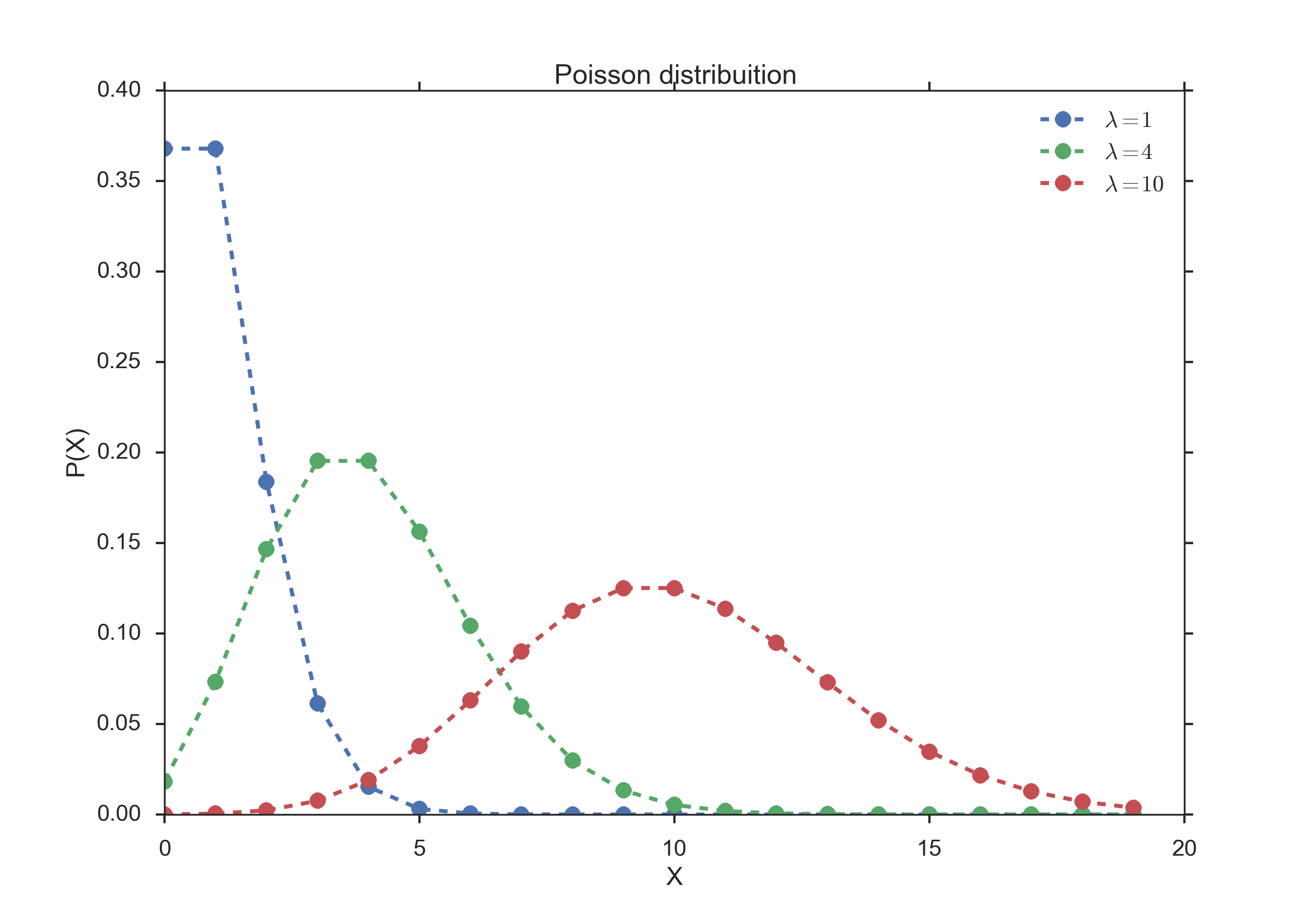
Poisson Distribution

Programs: Discrete Distribution Functions

32_figs_DistDiscrete.ipynb

Exercises

Numpy

1. Create an numpy-array, containing the data 1,2,3,...,10.

2. Calculate mean and sample(!)-standard deviation.

   (Correct answer: 3.03)

Distributions

1. Generate and plot the Probability Density Function (PDF) of a normal distribution, with a mean of 5 and a standard deviation of 3.

2. Generate 1000 random data from this distribution.

3. Calculate the standard error of the mean of these data. (Correct answer: ca. 0.096)

4. Plot the histogram of these data.

5. From the PDF, calculate the interval containing 95% of these data.

   (Correct answer: [ -0.88, 10.88])

Continuous Distributions

1. Normal Distribution: Your doctor tells you that he can use hip implants for surgery even if they are 1 mm bigger or smaller than the specified size. And your financial officer tells you that you can discard 1 out of 1000 hip implants, and still make a profit.

   What is the required standard deviation for the producer of the hip implants, to simultaneously satisfy both requirements? (Correct answer: SD = 0.304 mm)

2. T-Distribution: Measuring the weight of your collogues, you have obtained the following weights: 52, 70, 65, 85, 62, 83, 59 kg. Calculate the corresponding mean, and the 99% confidence interval for the mean. Note: with n values you have n-1 DOF for the t-distribution. (Correct answer: 68.0 +/- 17.2 kg)

3. Chi-square Distribution Create 3 normally distributed datasets (mean = 0, SD = 1), with 1000 samples each. Then square them, sum them (so that you have 1000 data-points), and create a histogram with 100 bins. This should be similar to the curve for the Chi-square distribution, with 3 DOF (i.e. it should come down at the left).

4. F Distribution You have two apple trees. There are three apples from the first tree that weigh 110, 121 and 143 grams respectively, and four from the other which weigh 88, 93, 105 and 124 grams respectively. Are the variances from the two trees different? Note: calculate the corresponding F-value, and check if the CDF for the corresponding F-distribution is <0.025. (Correct answer: no)

5. Binomial Distribution “According to research, pure blue eyes in Europe approach greatest frequency in Finland, Sweden and Norway(at 72%), followed by Estonia, Denmark(69%); Latvia, Ireland(66%); Scotland(63%); Lithuania(61%); The Netherlands(58%); Belarus, England(55%); Germany(53%); Poland, Wales(50%); Russia, The Czech Republic(48%); Slovakia(46%); Belgium(43%); Austria, Switzerland, Ukraine(37%); France, Slovenia(34%); Hungary(28%); Croatia(26%); Bosnia and Herzegovina(24%); Romania(20%); Italy(18%); Serbia, Bulgaria(17%); Spain(15%); Georgia, Portugal(13%); Albania(11%); Turkey and Greece(10%). Further analysis shows that the average occurrence of blue eyes in Europe is 34%, with 50% in Northern Europe and 18% in Southern Europe.”

   If we have 15 Austrian students in the class-room, what ist the chance of finding 3, 6, or 10 students with blue eyes?

   (Correct answer: 9%, 20.1%, and 1.4%)

6. Poisson Distribution On the streets of Austria there were 62 fatal accidents in 2012. Assuming that those are evenly distributed, we have on average 62 /(365/7)=1.19 fatal accidents per week. How big is the chance that in a given week there are no, 2, or 5 accidents? (Correct answer: 30.5%, 21.5%, 0.6%)