Getting Started

There are three reasons why I have decided to use Python for this lecture.

1. It is the most elegant programming language that I know.
2. It is free.
3. It is powerful.

I have not seen many books on Python that I really liked. My favorite introductory book is . D. Harms and K. McDonald. The Quick Python Book (2nd Ed). Manning Publications Co., 2010.

There are also many tutorials available on the internet (see links below). Personally, most of the time I just google; thereby I stick primarily a) to the official pages, and b) to http://stackoverflow.com/. Also, I have found user groups surprisingly active and helpful!

Python Links

• Python Scientific Lecture Notes. If you don’t read anything else, read this!
• NumPy for Matlab Users Start here if you have Matlab experience.
• Lectures on scientific computing with Python. Great IPython notebooks, from JR Johansson!
• The Python tutorial. The official introduction.

Free Python Books

• A Byte of Python. Free book, very good at the introductory level.
• Learn Python the Hard Way, 3rd Ed A popular, free book that you can work through.
• ThinkPython. Free book, for advanced programmers.
• Introduction to Python for Econometrics, Statistics and Data Analysis (pdf) by Kevin Sheppard: A good free book, which introduces Python with a focus on statistics.

Installation and Updates

In general, I suggest that you start out by installing a Python distribution which includes the most important libraries. Unless you have a specific requirement for 64-bit versions, I recommend that you install a 32-bit version of Python: it facilitates many activities that require compilation of module parts, e.g. for Bayesian statistics (PyMC), or when you want to speed up your programs with Cython. Since all the Python packages required for this course are now available for Python 3.x, I will use primarily Python 3 for this book. However, all the scripts included should also work for Python 2.7. My favorite Python distributions are

1. WinPython No admin-rights required. Recommended for Windows users.
2. anaconda From Continuum. For Windows, Mac, and Linux.

which are very good starting points when you are using Windows. winpython does not require administrator rights, and anaconda is a more recent distribution, which is free for educational purposes.

Mac and Unix users should check out the installations tips from Johansson.

PyPI - the Python Package Index

If you decide to install things manually, you need the following modules in addition to the Python standard library (in brackets I give the version number with which the code provided here was tested):

• ipython 2.3.0 ... For interactive work.
• numpy 1.9.1 ... For working with vectors and arrays.
• scipy 0.14.1 ... All the essential scientific algorithms, including those for statistics.
• matplotlib 1.4.2 ... The de-facto standard module for plotting and visualization.
• pandas 0.15.2 ... Adds DataFrames (imagine powerful spreadsheets) to Python.
• patsy 0.3.0 ... For working with statistical formulas.
• statsmodels 0.6.1 ... For statistical modeling and advanced analysis.
• seaborn 0.5.1 ... For visualization of statistical data.
• PyMC 2.3.4 ... For Bayesian statistics, including Markov chain Monte Carlo simulations.
• scikits.bootstrap 0.3.2 ... Provides bootstrap confidence interval algorithms for scipy.

The Python Package Index (*PyPI*) is a repository of software for the Python programming language. There are currently 53955 packages here!

To use a package from this index you simply can use

pip install [package]

and to update packages

pip install [package] -U

To get a list of all the Python packages installed, type

pip list

IPython

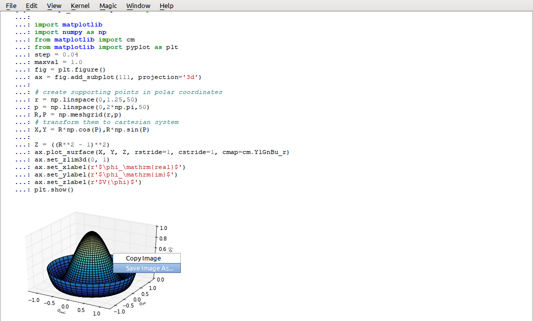
The “ipython qtconsole” provides a powerful and flexible interactive work environment.

Make sure that you have a good programming environment! Currently, my favorite way of programming is similar to my old Matlab style: I first get the individual steps worked out interactively in an ipython qtconsole. Ipython provides interactive computing with Python, similar to the commandline in Matlab. It comes with a command history, interactive data visualization, command completion, and a lot of features that make it quick and easy to try out code. When ipython is started in pylab mode (which is the typical configuration), it automatically loads numpy and matplotlib.pyplot into the active workspace, and provides a very convenient, Matlab-like programming environment.

A very helpful new addition is the browser-based ipython notebook, with support for code, text, mathematical expressions, inline plots and other rich media. Please check out the links to the ipython notebooks in this statistics introduction. I believe that it will help you to get up to speed with python much more quickly.

Personalizing IPython

When working on a new problem, I always start out with IPython. Once I have the individual steps working, I use the IPython command %history to get the commands I have used, and switch to an integrated development environment (typically Wing or Spyder).

To start up IPython quickly in the location and with the configuration I like, I use the following tricks (the following are the steps on MS Windows, but should be easy to adapt to other operating systems):

To personalize ipython, generate your own profile:

• run “cmd”

• In the newly created command shell, execute the following command

  ipython profile create $<myName>$
  

  (This generates a folder \(.ipython \backslash profile\_<myName> \backslash startup"\))

• Into this folder, place a file with e.g. the name \(00\_<myName>.py\), containing

  import pandas as pd
  import os
  os.chdir(r'C:\<your_favorite_dir>')"
  

• Generate a file “ipython.bat” in your startup-directory, containing

  [Python-directory]\backslash Scripts \backslash ipython3 qtconsole --profile <myName> --pylab=inline
  

Now you can start “your” ipython by just typing “ipython” in the Windows run command

To see all ipython notebooks for the course, do the following:

• run “cmd”

• Run the commands

  cd [ipynb-directory]
  [Python-directory]\backslash Scripts \backslash ipython3.exe notebook --pylab=inline
  

IPython Tips

1. Use pylab: ipython qtconsole —pylab=inline
2. For help on e.g. plot, use plot? or help(plot).
3. Check out the help tips when you start ipython.
4. Customize ipython on your computer: it will save you time in the long run!
5. TAB-completion, for file- and directory names, variable names, AND for commands
6. To switch between inline and external graphs, use %matplotlib inline and %matplotlib qt4
7. Use %runfile [aFile] to run a file, and import [aFile] to import it

Developing Python Programs

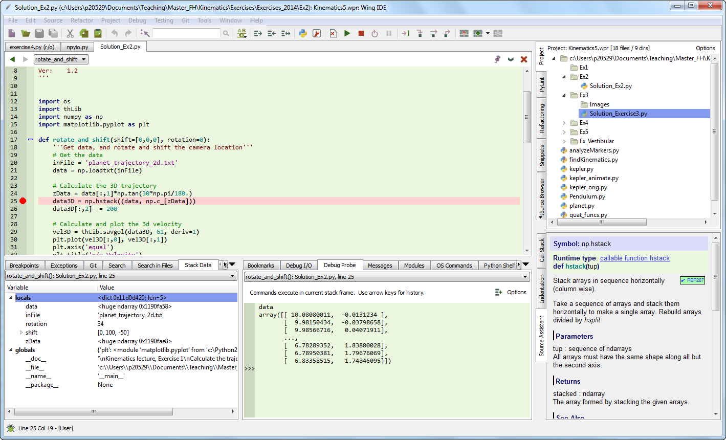
“Wing” is my favorite development environment, with probably the best existing debugger for Python.

To write a program, I typically take the commands I have worked out in ipython with %history, and take them to an IDE (integrated development environment): I either use Wing (my clear favorite Python IDE, although it is commercial) or Spyder (which is good and free). PyCharm is another IDE with a good debugger, and has very good vim-emulation.

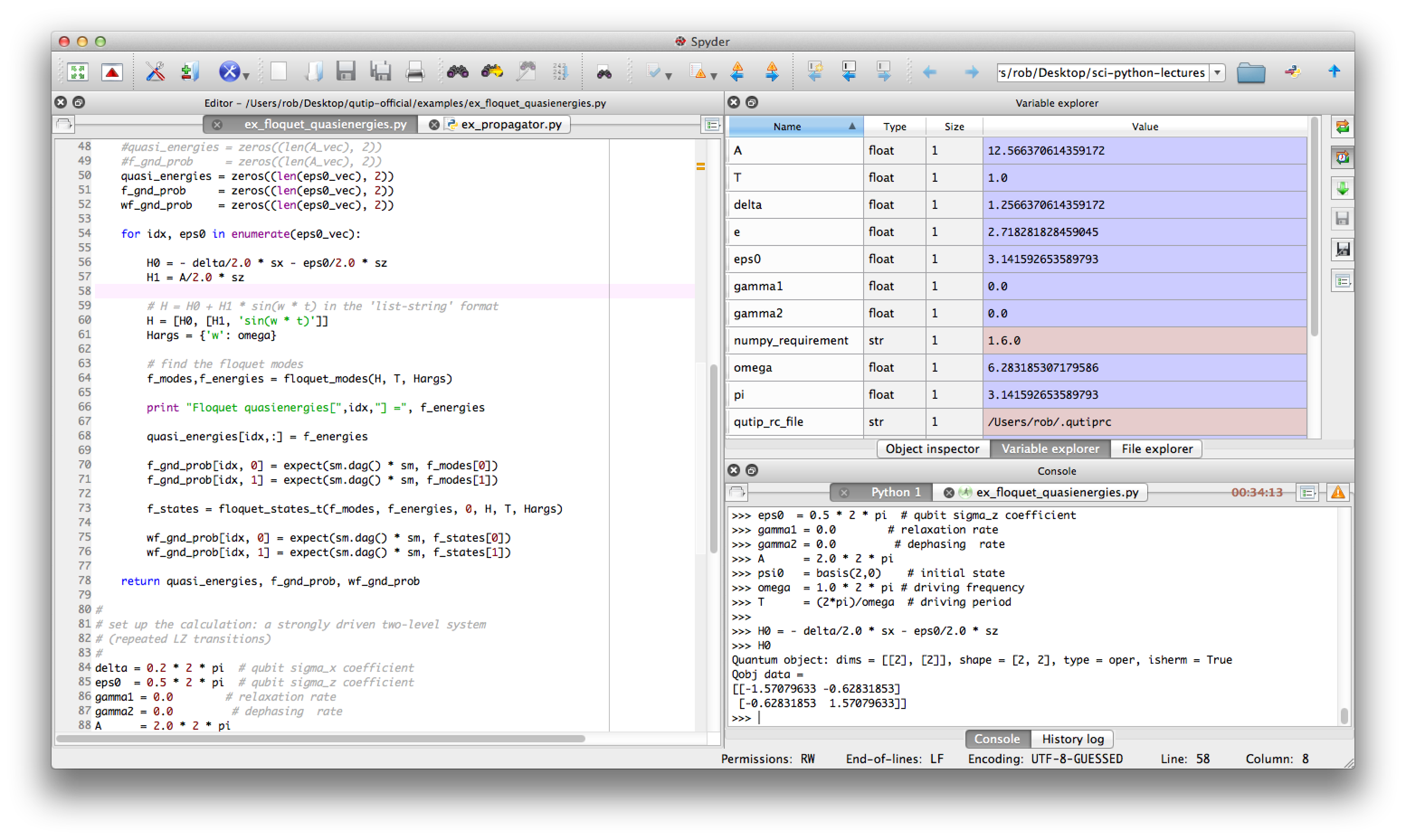
“Spyder” is a very good, free IDE.

Python Tips

1. Stick to the standard conventions.

   • Every function has a docu-string.

   • import matplotlib.pyplot as plt

     import numpy as np

     import scipy as sp

     import pandas as pd

     import seaborn as sns

2. To get the current directory, use os.path.abspath(os.curdir).

3. Everything in Python is an object: to find out about “obj”, use type(obj) and dir(obj).

4. Learn to use the debugger.

5. Know lists, tuples, and dictionaries; also, know about numpy arrays and pandas DataFrames.

6. Use functions a lot, and understand the if __name__=="__main__": construct.

Python Data Structures

Tuple ()

A collection of different things. Cannot be modified after creation.

List [

] A collection of similar things. Does not care if those are numbers or strings.

Array [

] Vectors and matrices, for numerical data manipulation. Defined in numpy.

Dictionary {}

Dictionaries are unordered (key/value) collections of content, where the content is addressed as dict[“key”] (see example below).

DataFrame

Data structure optimized for working with named, statistical data. Defined in pandas. (See next chapter.)

In [1]: myTuple = ('abc', np.arange(0,3,0.2), 2.5)

In [2]: myTuple[2]
Out[2]: 2.5

In [3]: myList = ['abc', 'def', 'ghij']

In [4]: myList.append('klm')

In [5]: myList2 = [1,2,3]

In [6]: myList3 = [4,5,6]

In [7]: myList2 + myList3
Out[7]: [1, 2, 3, 4, 5, 6]

In [8]: myArray = np.array(myList2)

In [9]: myArray2 = np.array(myList3)

In [10]: myArray + myArray2
Out[10]: array([5, 7, 9])

In [11]: myDict = dict(one=1, two=2, info='some information')

In [12]: myDict2 = {'ten':1, 'twenty':20, 'info':'more information'}

In [13]: myDict['info']
Out[13]: 'some information'

In [14]: myDict.keys()
Out[14]: dict_keys(['one', 'info', 'two'])

Matplotlib, pylab, and pyplot: how are they related?

The flexibility of Python has the “disadvantage” that it can come in different flavors or coding styles. When you know the different approaches, they are great to use. But when you get started, it can be a bit confusing. The following section from the Matplotlib documentation may help to clarify these things:

Matplotlib is the whole package; pylab is a Matlab-like module in matplotlib that gets installed alongside matplotlib; and matplotlib.pyplot is a module in matplotlib.

Pyplot provides the state-machine interface to the underlying plotting library in matplotlib. This means that figures and axes are implicitly and automatically created to achieve the desired plot. For example, calling plot from pyplot will automatically create the necessary figure and axes to achieve the desired plot. Setting a title will then automatically set that title to the current axes object:

import matplotlib.pyplot as plt

plt.plot(np.arange(10))
plt.title("Simple Plot")
plt.show()

Pylab combines the pyplot functionality (for plotting) with the numpy functionality (for mathematics and for working with arrays) in a single namespace, making that namespace (or environment) even more MATLAB-like. For example, one can call the sin and cos functions just like you could in MATLAB, as well as having all the features of pyplot.

The pyplot interface is generally preferred for non-interactive plotting (i.e., scripting). The pylab interface is convenient for interactive calculations and plotting, as it minimizes typing. Note that this is what you get if you use the ipython shell with the -pylab option, which imports everything from pylab and makes plotting fully interactive.

Coding Styles in Python

In Python you will find different coding styles and usage patterns. These styles are all perfectly valid, and each have their pros and cons. Just about all of the examples can be converted into another style and achieve the same results. The only caveat is to avoid mixing the coding styles for your own code.

Of the different styles, there are two that are officially supported. Therefore, these are the preferred ways to use matplotlib.

For the preferred pyplot style, the imports at the top of your scripts will typically be:

import matplotlib.pyplot as plt
import numpy as np

Then one calls, for example, np.arange, np.zeros, np.pi, plt.figure, plt.plot, plt.show, etc. So, a simple example in this style would be:

import matplotlib.pyplot as plt
import numpy as np
x = np.arange(0, 10, 0.2)
y = np.sin(x)
plt.plot(x, y)
plt.show()

Note that this example used pyplot”s state-machine to automatically and implicitly create a figure and an axes. For full control of your plots and more advanced usage, use the pyplot interface for creating figures, and then use the object methods for the rest:

import matplotlib.pyplot as plt
import numpy as np
x = np.arange(0, 10, 0.2)
y = np.sin(x)
fig = plt.figure()
ax = fig.add_subplot(111)
ax.plot(x, y)
plt.show()

Next, the same example using a pure MATLAB-style:

from pylab import *
x = arange(0, 10, 0.2)
y = sin(x)
plot(x, y)

So, why all the extra typing as one moves away from the pure MATLAB-style? For very simple things like this example, the only advantage is academic: the wordier styles are more explicit, more clear as to where things come from and what is going on. For more complicated applications, this explicitness and clarity becomes increasingly valuable, and the richer and more complete object-oriented interface will likely make the program easier to write and maintain.

Here an example, to get you started with Python. For interactive work, it is simplest to use the pylab mode, as shown in the example below.

Example-Session

10_getting_started.ipynb gives a short demonstration of Python for scientific data analysis.

Pandas

pandas is a Python module which provides suitable data structures for statistical analysis. It significantly enhances the abilities of Python for data input, data organization, and data manipulation. In the following, I assume that pandas has been imported with

import pandas as pd

A good introduction to pandas can be found under http://www.randalolson.com/2012/08/06/statistical-analysis-made-easy-in-python/

Data Input

Pandas offers tools for reading and writing data between in-memory data structures and different formats, e.g. CSV and text files, Microsoft Excel, and SQL databases. For example, if you have data in your clipboard, you can import them directly with

data = pd.read_clipboard()

Or data from “Sheet1” in an Excel-file “data.xls” can be read in easily with

xls = pd.io.parsers.ExcelFile('data.xls')
data = xls.parse('Sheet1')

Example: readZip.py This advanced script shows you how you can directly import data from an MS-Excel file from a zipped archive on the web.

Data Handling and Manipulation

To handle labeled data, pandas introduces DataFrame objects. A DataFrame is a 2-dimensional labeled data structure with columns of potentially different types. You can think of it like a spreadsheet or SQL table. It is generally the most commonly used pandas object. At first, handling data with Pandas feels a bit unusual. To get you started, let me give you a specific example:

import numpy as np
import pandas as pd

t = np.arange(0,10,0.1)
x = np.sin(t)
y = np.cos(t)

df = pd.DataFrame({'Time':t, 'x':x, 'y':y})

In Pandas, rows are addressed through “indices”, and columns through their “column” name. To address the first column only, you have two options:

df.Time
df['Time']

If you want to extract two columns at the same time, you have to use a Python-list:

data = df[['Time', 'y']]

To display the first or last rows, use

data.head()
data.tail()

For e.g. rows 5-10 (note that this are 6 numbers), use

data[4:10]

as \(10-4=6\). (I know, the array indexing takes some time to get used to. Just keep in mind that Python addresses the locations between entries, not the entries, and that it starts at \(0\)!!) To do this in one go, use

df[['Time', 'y']][4:10]

You can also apply the standard row/column notation, by using the method “ix”:

df.ix[[0,2],4:10]

Finally, sometimes you want to have direct access to the data, not to the DataFrame. You can do this with

data.values

Pandas offers powerful functions to handle missing data and “nans”, and other kinds of data manipulation like pivoting. For example, you can use data-frames to efficiently group objects, and do a statistical evaluation of each group. The following data are simulated (but realistic) data of a survey on how many hours a day people watch on the TV, grouped into “m”ale and “f”emale responses:

data = pd.DataFrame({
    'Gender': ['f', 'f', 'm', 'f', 'm', 'm', 'f', 'm', 'f', 'm'],
    'TV': [3.4, 3.5, 2.6, 4.7, 4.1, 4.0, 5.1, 4.0, 3.7, 2.1]
    })

# Group the data
grouped = data.groupby('Gender')

# Get the groups as DataFrames
df_female = grouped.get_group('f')

# Get the corresponding numpy-array
values_female = grouped.get_group('f').values

# or equivalently
groups = grouped.groups
values_female = groups['f']

# Do some overview statistics
print(grouped.describe())

produces

                    TV
Gender
f      count  5.000000
       mean   4.080000
       std    0.769415
       min    3.400000
       25%    3.500000
       50%    3.700000
       75%    4.700000
       max    5.100000
m      count  5.000000
       mean   3.360000
       std    0.939681
       min    2.100000
       25%    2.600000
       50%    4.000000
       75%    4.000000
       max    4.100000

For statistical analysis, pandas becomes really powerful if you combine it with statsmodels (see below).

Statsmodels

statsmodels is a Python module that provides classes and functions for the estimation of many different statistical models, as well as for conducting statistical tests, and statistical data exploration. An extensive list of result statistics are available for each estimator. statsmodels also allows the formulation of models with the popular formula language also used by \(R\), the leading statistics package. For example, data on the connection between academic “success”, “intelligence” and “diligence” can be described with the model

\[success \sim intelligence * diligence\]

which would capture the direct effect of “intelligence” and “diligence”, as well as the interaction. You find more information on that topic in the section “Statistical Models”.

While for complex statistical models R still has an edge, python has a much clearer and more readable syntax, and is arguably more powerful for the data manipulation often required for statistical analysis.

11_statsmodels_intro.ipynb shows you how the combination of pandas and statsmodels can be used for data analysis.

Seaborn

seaborn is a Python visualization library based on matplotlib. Its primary goal is to provide a concise, high-level interface for drawing statistical graphics that are both informative and attractive.

x = linspace(1, 7, 50)
y = 3 + 2*x + 1.5*randn(len(x))
sns.regplot(x,y)

already produces a nice and informative regression plot (Fig. below).

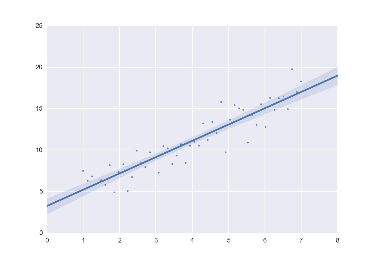
Regression plot, from “seaborn”, with a substantial amount of added information.

Exercises

• Read in data from different sources:
  • A CVS-file with a header (“Data\data_kaplan\swim100m.csv”)
  • An MS-Excel file (“Data\data_others\Table 6.6 Plant experiment.xls”)
  • Data from the WWW (see “readZip.py” [py:readZip])
• • Generate a pandas dataframe, with the x-column time stamps from 0 to 10 sec, at a rate of 10 Hz, the y-column data values with a sine with 1.5 Hz, and the z-column the corresponding cosine values. Label the x-column “Xvals”, and the y-column “YVals”, and the z-column “ZVals”.
  • Show the head of this dataframe
  • Extract the data in lines 10-15 from “Yvals” and “ZVals”, and write them to the file “out.txt”.