There is a substantial difference in approach between hypothesis tests and statistical modeling. In the former case, you typically start out with a null hypothesis. Based on your question and your data, you then select the appropriate statistical test as well as the desired significance level, and either accept or reject the null hypothesis.

In contrast, statistical modeling is much more an interactive analysis of the data. Based on a first look at the data, you typically start out with selecting a statistical model that may describe your data. In the previous chapters, we have for example described the hypythesized linear relationship between data with the model

\[y = k*x + d\]

You then

determine the model parameters (e.g. k and d),
assess the quality of the model (e.g. through the $R^2$-value, or another suitable parameter),
and inspect the residuals, to check if your proposed model has missed essential features in the data.

If you are not happy with the quality of the model, or if you find during the inspection of the residuals that you have either outliers or need another model, you modify your proposed model and repeat this procedure until you are happy with the results. You see that in comparison to hypothesis tests, statistical modeling involves much more an interactive playing with the data.

Model language¶

The mini-language commonly used now in statistics to describe formulas was first used in the languages $R$ and $S$, but is now also available in Python through the module patsy.

For instance, if we have some variable $y$, and we want to regress it against some other variables $x, a, b$, and the interaction of a and b, then we simply write

\[y \sim x + a + b + a:b\]

The symbols in Table are used on the right hand side to denote different interactions.

A complete set of the description is found under http://patsy.readthedocs.org/

Design Matrix¶

Definition¶

A very general definition of a regression model is the following:

\[\label{eq:regmodel} Y = f(x,\varepsilon)\]

In the case of a linear regression model, the function f is simply the affine function, and the model can be rewritten as:

\[\label{eq:simplereg} Y = X \beta + \varepsilon\]

For a simple linear regression and multivariate regression, the corresponding Design Matrices are given in the sections on simple linear regression and on multivariate regression.

Given a data set $\{y_i,\, x_{i1}, \ldots, x_{ip}\}_{i=1}^n$ of $n$ statistical units, a linear regression model assumes that the relationship between the dependent variable $y_i$ and the $p$-vector of regressors $x_i$ is linear. This relationship is modelled through a disturbance term or error variable $\epsilon_i$, an unobserved random variable that adds noise to the linear relationship between the dependent variable and regressors. Thus the model takes the form

\[\label{eq:regression} y_i = \beta_1 x_{i1} + \cdots + \beta_p x_{ip} + \varepsilon_i = \mathbf{x}^{\rm T}_i \beta + \varepsilon_i, \qquad i = 1, \ldots, n,\]

where $^T$ denotes the transpose, so that $x_i^T\beta$ is the inner product between vectors $x_i$ $\beta$.

Often these $n$ equations are stacked together and written in vector form as

\[\mathbf{y} = \mathbf{X}\beta + \varepsilon, \,\]

where

\[\begin{split}\mathbf{y} = \begin{pmatrix} y_1 \\ y_2 \\ \vdots \\ y_n \end{pmatrix}, \quad \mathbf{X} = \begin{pmatrix} \mathbf{x}^{\rm T}_1 \\ \mathbf{x}^{\rm T}_2 \\ \vdots \\ \mathbf{x}^{\rm T}_n \end{pmatrix} = \begin{pmatrix} x_{11} & \cdots & x_{1p} \\ x_{21} & \cdots & x_{2p} \\ \vdots & \ddots & \vdots \\ x_{n1} & \cdots & x_{np} \end{pmatrix}, \quad \beta = \begin{pmatrix} \beta_1 \\ \vdots \\ \beta_p \end{pmatrix}, \quad \varepsilon = \begin{pmatrix} \varepsilon_1 \\ \varepsilon_2 \\ \vdots \\ \varepsilon_n \end{pmatrix}.\end{split}\]

Some remarks on terminology and general use:

$y_i$ is called the regressand, endogenous variable, response variable, measured variable, or dependent variable. The decision as to which variable in a data set is modeled as the dependent variable and which are modeled as the independent variables may be based on a presumption that the value of one of the variables is caused by, or directly influenced by the other variables. Alternatively, there may be an operational reason to model one of the variables in terms of the others, in which case there need be no presumption of causality.
$\mathbf{x}_i$ are called regressors, exogenous variables, explanatory variables, covariates, input variables, predictor variables, or independent variables, but not to be confused with independent random variables. The matrix $\mathbf{X}$ is sometimes called the design matrix.
- Usually a constant is included as one of the regressors. For example we can take $x_{i1}=1$ for $i=1,...,n$. The corresponding element of $\beta$ is called the intercept. Many statistical inference procedures for linear models require an intercept to be present, so it is often included even if theoretical considerations suggest that its value should be zero.
- Sometimes one of the regressors can be a non-linear function of another regressor or of the data, as in polynomial regression and segmented regression. The model remains linear as long as it is linear in the parameter vector $\beta$.
- The regressors $x_{ij}$ may be viewed either as random variables, which we simply observe, or they can be considered as predetermined fixed values which we can choose. Both interpretations may be appropriate in different cases, and they generally lead to the same estimation procedures; however different approaches to asymptotic analysis are used in these two situations.
$\beta\,$ is a $p$-dimensional parameter vector. Its elements are also called effects, or regression coefficients. Statistical estimation and inference in linear regression focuses on $\beta$.
$\varepsilon_i\,$ is called the residuals, error term, disturbance term, or noise. This variable captures all other factors which influence the dependent variable $y_i$ other than the regressors $x_i$. The relationship between the error term and the regressors, for example whether they are correlated, is a crucial step in formulating a linear regression model, as it will determine the method to use for estimation.
If $i=1$ and $p=1$ in the equation above, we have a simple linear regression, corresponding to $y = k*x + d + \epsilon$ . If $i>1$ we talk about multilinear regression or multiple linear regression .

Example. Consider a situation where a small ball is being tossed up in the air and then we measure its heights of ascent $h_i$ at various moments in time $t_i$. Physics tells us that, ignoring the drag, the relationship can be modelled as :

\[h_i = \beta_1 t_i + \beta_2 t_i^2 + \varepsilon_i,\]

where $\beta_1$ determines the initial velocity of the ball, $\beta_2$ is proportional to the standard gravity, and $\epsilon_i$ is due to measurement errors. Linear regression can be used to estimate the values of $\beta_1$ and $\beta_2$ from the measured data. This model is non-linear in the time variable, but it is linear in the parameters $\beta_1$ and $\beta_2$; if we take regressors $\mathbf{x}_i = (x_{i1},x_{i2}) = (t_i,t_i^2)$, the model takes on the standard form : $h_i = \mathbf{x}^{\rm T}_i\beta + \varepsilon_i.$

Examples¶

One-way ANOVA (Cell Means Model)¶

Example with a one-way analysis of variance (ANOVA) with 3 groups and 7 observations. The given data set has the first three observations belonging to the first group, the following two observations belong to the second group and the final two observations are from the third group. If the model to be fit is just the mean of each group, then the model is

\[y_{ij} = \mu_i + \epsilon_{ij}\]

which can be written

\[\begin{split}\begin{bmatrix}y_1 \\ y_2 \\ y_3 \\ y_4 \\ y_5 \\ y_6 \\ y_7 \end{bmatrix} = \begin{bmatrix}1 & 0 & 0 \\1 &0 &0 \\ 1 & 0 & 0 \\ 0 & 1 & 0 \\ 0 & 1 & 0 \\ 0 & 0 & 1 \\ 0 & 0 & 1\end{bmatrix} \begin{bmatrix}\mu_1 \\ \mu_2 \\ \mu_3 \end{bmatrix} + \begin{bmatrix} \epsilon_1 \\ \epsilon_2 \\ \epsilon_3 \\ \epsilon_4 \\ \epsilon_5 \\ \epsilon_6 \\ \epsilon_7 \end{bmatrix}\end{split}\]

It should be emphasized that in this model $\mu_i$ represents the mean of the $i$th group.

One-way ANOVA (offset from reference group)¶

The ANOVA model could be equivalently written as each group parameter $\tau_i$ being an offset from some overall reference. Typically this reference point is taken to be one of the groups under consideration. This makes sense in the context of comparing multiple treatment groups to a control group and the control group is considered the “reference”. In this example, group 1 was chosen to be the reference group. As such the model to be fit is:

\[y_{ij} = \mu + \tau_i + \epsilon_{ij}\]

with the constraint that $\tau_1$ is zero.

\[\begin{split}\begin{bmatrix}y_1 \\ y_2 \\ y_3 \\ y_4 \\ y_5 \\ y_6 \\ y_7 \end{bmatrix} = \begin{bmatrix}1 &0 &0 \\1 &0 &0 \\ 1 & 0 & 0 \\ 1 & 1 & 0 \\ 1 & 1 & 0 \\ 1 & 0 & 1 \\ 1 & 0 & 1\end{bmatrix} \begin{bmatrix}\mu \\ \tau_2 \\ \tau_3 \end{bmatrix} + \begin{bmatrix} \epsilon_1 \\ \epsilon_2 \\ \epsilon_3 \\ \epsilon_4 \\ \epsilon_5 \\ \epsilon_6 \\ \epsilon_7 \end{bmatrix}\end{split}\]

In this model $\mu$ is the mean of the reference group and $\tau_i$ is the difference from group $i$ to the reference group. $\tau_1$ and is not included in the matrix because its difference from the reference group (itself) is necessarily zero.

Example 1: Program Effectiveness¶

In this rather simple example we use data from Spector and Mazzeo (1980), to estimate a linear regression model with statsmodels.

'''Linear Regression
Estimation of a linear regression model using the Spector and Mazzeo (1980) data set.

Documentation:
    data on 32 students TUCE scores
    5 columns with rows = students

    1) Grade ..... post grade
    2) constant .. term
    3) psi
    4) tuce ...... tuce (test of understanding of college economics) score
    5) gpa ....... grade point average

'''

'''
Author: Bruno Rodrigues
Date:   March-2013
Ver:    1.3 (Thomas Haslwanter)
'''

# Linked to text in: An Introduction to Statistics
# For this we only need to import statsmodels
import statsmodels.api as sm

def main():
    # We load the spector dataset as a pandas dataframe
    # Of course, you can load your own datasets 
    data = sm.datasets.spector.load_pandas()
    
    # We define y as the endogenous variable, and x as the 
    # exogenous variable.
    # Note that if you load your own data, the methods endog 
    # and exog will not be available and you will have to 
    # explicitly define the endogenous and exogenous variables
    y, x = data.endog, data.exog
    
    # We do the regression
    reg = sm.OLS(y, x).fit()
    
    # And here we can see the results in a very nice looking table
    print('SUMMARY -------------------------------------------')
    print((reg.summary()))
    
    # We can only take a look at the parameter values though
    print('PARAMETERS ----------------------------------------')
    print((reg.params))
    
    # We can also extract the residuals
    print('RESIDUALS -----------------------------------------')
    print((reg.resid))
    
    # This line is just to prevent the output from vanishing when you
    # run the program by double-clicking
    input('Done - Hit any key to finish.')

if __name__ == '__main__':
    main()

Example 2: Linear Models¶

This second set of examples is based heavily on Jonathan Taylor’s class notes that use R. The following notebook introduces the use of pandas and the formula framework in statsmodels in the context of linear modeling:

Ipython notebook 100_statsIntro_linearModels.ipynb

Linear Regression Analysis with Python¶

The following is based on the blog of Connor Johnson.

We will use Python to explore measures of fit for linear regression: the coefficient of determination ($R^2$), hypothesis tests (F, t, Omnibus), AIC, BIC, and other measures.

First we will look at a small data set from DASL library, regarding the correlation between tobacco and alcohol purchases in different regions of the United Kingdom. The interesting feature of this data set is that Northern Ireland is reported as an outlier. Notwithstanding, we will use this data set to describe two tools for calculating a linear regression. We will alternatively use the statsmodels and sklearn modules for calculating the linear regression, while using pandas for data management, and matplotlib for plotting. To begin, we will import the modules, get the data into Python, and have a look at them:

import numpy as np
import pandas as pd
import matplotlib.pyplot as plt
import statsmodels.formula.api as sm
from sklearn.linear_model import LinearRegression
from scipy import stats

data_str = '''Region Alcohol Tobacco
North 6.47 4.03
Yorkshire 6.13 3.76
Northeast 6.19 3.77
East_Midlands 4.89 3.34
West_Midlands 5.63 3.47
East_Anglia 4.52 2.92
Southeast 5.89 3.20
Southwest 4.79 2.71
Wales 5.27 3.53
Scotland 6.08 4.51
Northern_Ireland 4.02 4.56'''

# Read in the data. Note that for Python 2.x, you have to change the "import" statement
from io import StringIO
df = pd.read_csv(StringIO(data_str), sep=r'\s+')

# Plot the data
df.plot('Tobacco', 'Alcohol', style='o')
plt.ylabel('Alcohol')
plt.title('Sales in Several UK Regions')
plt.show()

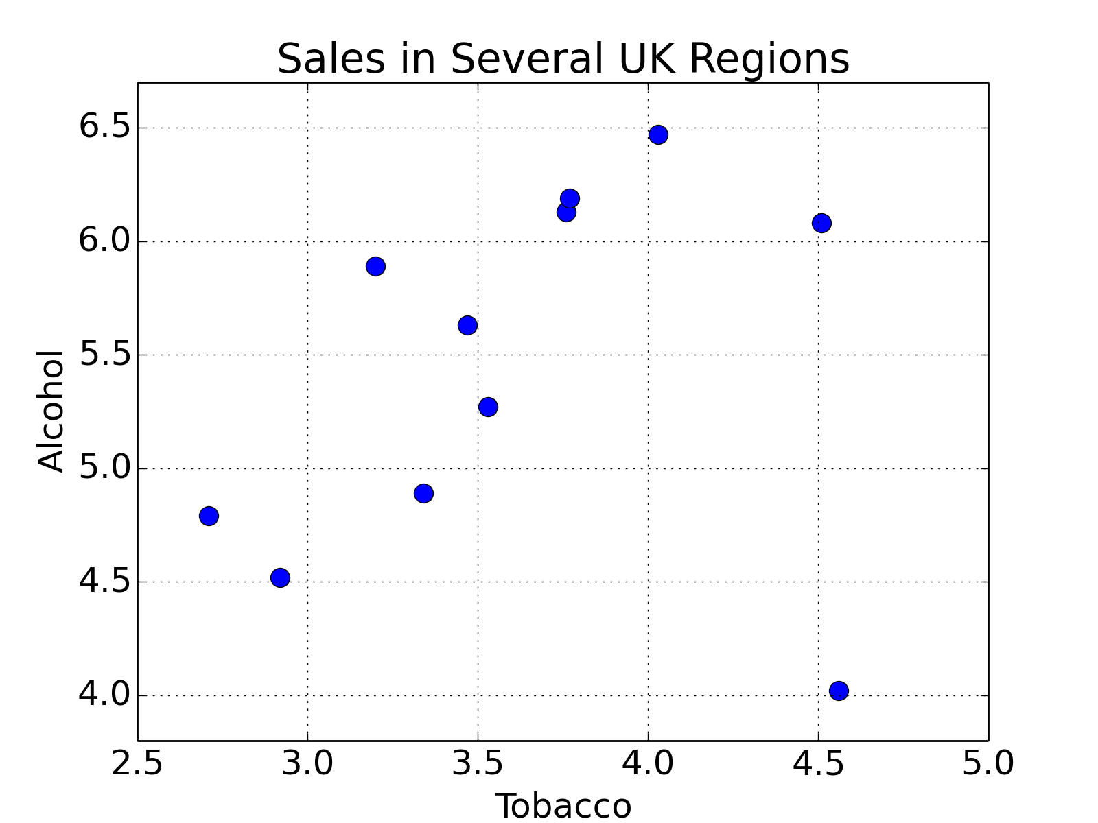
Sales of Alcohol vs Tobacco in the UK. We notice that there seems to be a linear trend, and one outlier, which corresponds to North Ireland.

Fitting the model, leaving the outlier for the moment away is then very easy:

result = smf.ols('Alcohol ~ Tobacco', df[:-1]).fit()
print(result.summary())

Note that using the formula API from statsmodels, an intercept is automatically added. This gives us

                            OLS Regression Results
==============================================================================
Dep. Variable:                Alcohol   R-squared:                       0.615
Model:                            OLS   Adj. R-squared:                  0.567
Method:                 Least Squares   F-statistic:                     12.78
Date:                Sun, 27 Apr 2014   Prob (F-statistic):            0.00723
Time:                        13:19:51   Log-Likelihood:                -4.9998
No. Observations:                  10   AIC:                             14.00
Df Residuals:                       8   BIC:                             14.60
Df Model:                           1
==============================================================================
                 coef    std err          t      P>|t|      [95.0% Conf. Int.]
------------------------------------------------------------------------------
Intercept      2.0412      1.001      2.038      0.076        -0.268     4.350
Tobacco        1.0059      0.281      3.576      0.007         0.357     1.655
==============================================================================
Omnibus:                        2.542   Durbin-Watson:                   1.975
Prob(Omnibus):                  0.281   Jarque-Bera (JB):                0.904
Skew:                          -0.014   Prob(JB):                        0.636
Kurtosis:                       1.527   Cond. No.                         27.2
==============================================================================

And now we have a very nice table of mostly meaningless numbers. I will go through and explain each one. The left column of the first table is mostly self explanatory. The degrees of freedom of the model are the number of predictor, or explanatory variables. The degrees of freedom of the residuals is the number of observations minus the degrees of freedom of the model, minus one (for the offset).

Most of the values listed in the summary are available via the result object. For instance, the $R^2$ value is obtained by result.rsquared. If you are using IPython, you may type result. and hit the TAB key, and a list of attributes for the result object will drop down.

Model Results¶

Definitions for Regression with Intercept¶

$n$ is the number of observations, $k$ is the number of regression parameters. For example, if you fit a straight line, $k=2$. In the following $\hat{y}_i$ will indicate the fitted model values, and $\bar{y}$ will indicate the mean.

$SS_\text{mod} = \sum_{i=1}^n (\hat{y}_i-\bar{y})^2$ is the Model Sum of Squares, or the sum of squares for the regression.
$SS_\text{res} = \sum_{i=1}^n (y_i-\hat{y}_i)^2$ is the Residuals Sum of Squares, or the sum of squares for the errors.
$SS_\text{tot} = \sum_{i=1}^n (y_i-\bar{y})^2$ is the Total Sum of Squares, and is equivalent to the sample variance multiplied by $n-1$.

For multiple regression models, $SS_\text{mod} + SS_\text{res} = SS_\text{tot}$

$DF_\text{mod} = k - 1$ is the (Corrected) ModelDegrees of Freedom . (The “-1” comes from the fact that we are only interested in the correlation, not in the absolute offset of the data.)
$DF_\text{res} = n - k$ is the Residuals Degrees of Freedom
$DF_\text{tot} = n - 1$ is the (Corrected) Total Degrees of Freedom. The Horizontal line regression is the null hypothesis model.

For multiple regression models with intercept, $DF_\text{mod} + DF_\text{res} = DF_\text{tot}$.

$MS_\text{mod} = SS_\text{mod} / DF_\text{mod}$ : Model Mean of Squares
$MS_\text{res} = SS_\text{res} / DF_\text{res}$ : Residuals Mean of Squares. $MS_\text{res}$ is an unbiased estimate for $\sigma^2$ for multiple regression models.
$MS_\text{tot} = SS_\text{tot} / DF_\text{tot}$ : Total Mean of Squares, which is the sample variance of the y-variable.

The $R^2$ Value¶

The $R^2$ value indicates the proportion of variation in the y-variable that is due to variation in the x-variables. For simple linear regression, the $R^2$ value is the square of the sample correlation $r_{xy}$. For multiple linear regression with intercept (which includes simple linear regression), the $R^2$ value is defined as

\[R^2 = \frac{SS_\text{mod}}{SS_\text{tot}}\]

$\bar{R}^2$ - The adjusted $R^2$ Value¶

Many researchers prefer the adjusted :math:`bar{R}^2` value, which is penalized for having a large number of parameters in the model:

Here is the logic behind the definition of $\bar{R}^2$: $R^2$ is defined as $R^2 = 1 - SS_\text{res}/SS_\text{tot}$ or $1 - R^2 = SS_\text{res}/SS_\text{tot}$. To take into account the number of regression parameters $p$, define the adjusted R-squared value as

\[1- \bar{R}^2 = \frac{ResidualVariance }{Total Variance}\]

where (Sample) Residual Variance is estimated by $SS_\text{res}/DF_\text{res} = SS_\text{res}/(n-k)$, and (Sample) Total Variance is estimated by $SS_\text{tot}/DF_\text{tot} = SS_\text{tot}/(n-1)$. Thus,

\[\begin{split}\begin{aligned} 1 - \bar{R}^2 &=& \frac{SS_\text{res}/(n - k)}{SS_\text{tot}/(n - 1)} \nonumber \\ &=& \frac{SS_\text{res}}{SS_\text{tot}}\frac{n - 1}{n - k}\end{aligned}\end{split}\]

so

\[\begin{split}\begin{aligned} \bar{R}^2 &=& 1 - \frac{SS_\text{res}}{SS_\text{tot}} \frac{n - 1}{n - k} \nonumber \\ &=& 1 - (1 - R^2)\frac{n - 1}{n - k}\end{aligned}\end{split}\]

The F-test¶

If $t_1, t_2, ... , t_m$ are independent, $N(0, \sigma^2)$ random variables, then $\sum_{i=1}^m \frac{t_i^2}{\sigma^2}$ is a $\chi^2$ (chi-squared) random variable with $m$ degrees of freedom.

For a multiple regression model with intercept,

\[Y_j = \alpha + \beta_1 X_{1j} + ... + \beta_n X_{nj} + \epsilon_i = \alpha + \sum_{i=1}^n \beta_i X_{ij} + \epsilon_j = E(Y_j | X) + \epsilon_j\]

we want to test the following null hypothesis and alternative hypothesis:

$H_0$: $\beta_1$ = $\beta_2$ = ... = $\beta_n$ = 0

$H_1$: $\beta_j \neq 0$, for at least one value of j

This test is known as the overall F-test for regression.

It can be shown that if $H_0$ is true and the residuals are unbiased, homoscedastic (i.e. all function values have the same variance), independent, and normal (see section [sec:Assumptions] ):

$SS_\text{res} / \sigma^2$ has a $\chi^2$ distribution with $DF_\text{res}$ degrees of freedom.
$SS_\text{mod} / \sigma^2$ has a $\chi^2$ distribution with $DF_\text{mod}$ degrees of freedom.
$SS_\text{res}$ and $SS_\text{mod}$ are independent random variables.

If $u$ is a $\chi^2$ random variable with $n$ degrees of freedom, $v$ is a $\chi^2$ random variable with $m$ degrees of freedom, and $u$ and $v$ are independent, then $F = \frac{u/n}{v/m}$ has an F distribution with $(n,m)$ degrees of freedom.

If H0 is true,

\[F = \frac{(SS_\text{mod}/\sigma^2)/DF_\text{mod}}{(SS_\text{res}/\sigma^2)/DF_\text{res}} = \frac{SS_\text{mod}/DF_\text{mod}}{SS_\text{res}/DF_\text{res}} = \frac{MS_\text{mod}}{MS_\text{res}},\]

has an F distribution with $(DF_\text{mod}, DF_\text{res})$ degrees of freedom, and is independent of $\sigma$.

We can test this directly in Python with

N = result.nobs
k = result.df_model+1
dfm, dfe = k-1, N - k
F = result.mse_model / result.mse_resid
p = 1.0 - stats.f.cdf(F,dfm,dfe)
print('F-statistic: {:.3f},  p-value: {:.5f}'.format( F, p ))

which gives us

F-statistic: 12.785,  p-value: 0.00723

Here, stats.f.cdf( F, m, n ) returns the cumulative sum of the F-distribution with shape parameters m = k-1 = 1, and n = N - k = 8, up to the F-statistic $F$. Subtracting this quantity from one, we obtain the probability in the tail, which represents the probability of observing F-statistics more extreme than the one observed.

Log-Likelihood Function¶

A very common approach in statistics is the idea of Maximum Likelihood estimation. The basic idea is quite different from the minimum square approach: there, the model is constant, and the errors of the response are variable; in contrast, in the maximum likelihood approach, the data response values are regarded as constant, and the likelihood of the model is maximised.

For the Classical Linear Regression Model (with normal errors) we have

\[\epsilon = y_i - \sum_{k=1}^n \beta_k x_{ik} = y_i - \hat{y}_i \; in \; N(0, \sigma^2)\]

so the probability density is given by

\[p(\epsilon_i) = \Phi (\frac{y_i - \hat{y}_i}{\sigma})\]

where $\Phi(z)$ is the standard normal probability distribution function. The probability of independent samples is the product of the individual probabilities

\[\Pi_{total} = \prod_{i=1}^n p(\epsilon_i)\]

The Log Likelihood function is defined as

\[\begin{split}\begin{aligned} ln(\mathfrak{L}) &=& ln(\Pi_{total}) \\ &=& ln\left[\prod_{i=1}^n \frac{1}{\sigma\sqrt{2 \pi}} \exp \left(\frac{(y_i - \hat{y}_i)^2}{2 \sigma^2}\right)\right] \\ &=& \sum_{i=1}^n\left[log\left(\frac{1}{\sigma \sqrt{2 \pi}}\right)- \left(\frac{(y_i - \hat{y}_i)^2}{2 \sigma^2}\right)\right]\end{aligned}\end{split}\]

It can be shown that the maximum likelihood estimator of $\sigma^2$ is

\[E(\sigma^2) = \frac{SSE}{n}\]

We can calculate this in Python as follows:

N = result.nobs
SSR = result.ssr
s2 = SSR / N
L = ( 1.0/np.sqrt(2*np.pi*s2) ) ** N * np.exp( -SSR/(s2*2.0) )
print('ln(L) =', np.log( L ))

>>> ln(L) = -4.99975869739

Information Content of Statistical Models - AIC and BIC¶

To judge the quality of your model, you should first visually inspect the residuals. In addition, you can also use a number of numerical criteria to assess the quality of a statistical model. These criteria represent various approaches for balancing model accuracy with parsimony.

We have already encountered the $adjusted\; R^2$ value (Eq [eq:adjustedR2]), which - in contrast to the $R^2$ value - decreases if there are too many regressors in the model.

Other commonly encountered criteria are the Akaike Information Criterion (AIC) and the Schwartz or Bayesian Information Criterion (BIC) , which are based on the log-likelihood described in the previous section. Both measures introduce a penalty for model complexity, but the AIC penalizes complexity less severely than the BIC. The Akaike Information Criterion AIC is given by

\[AIC = 2*k - 2*ln(\mathfrak{L})\]

and the Schwartz or Bayesian Information Criterion BIC by

\[BIC = k*ln(N) - 2*ln(\mathfrak{L})\]

are other commonly encountered criteria. Here, $N$ is the number of observations, $k$ is the number of parameters, and $\mathcal{L}$ is the likelihood. We have two parameters in this example, the slope and intercept. The AIC is a relative estimate of information loss between different models. The BIC was initially proposed using a Bayesian argument, and does not related to ideas of information. Both measures are only used when trying to decide between different models. So, if you have one regression for alcohol sales based on cigarette sales, and another model for alcohol consumption that incorporated cigarette sales and lighter sales, then you would be inclined to choose the model that had the lower AIC or BIC value.

Model Coefficients and Their Interpretation¶

Coefficients¶

The coefficients or weights of the linear regression are contained in result.params, and returned as a pandas Series object, since we used a pandas DataFrame as input. This is nice, because the coefficients are named for convenience.

result.params
>>> Intercept    2.041223
>>> Tobacco      1.005896
>>> dtype: float64

We can obtain this directly by computing

\[\beta = (X^{T}X)^{-1}X^{T}y.\]

Here, $X$ is the matrix of predictor variables as columns, with an extra column of ones for the constant term, $y$ is the column vector of the response variable, and $\beta$ is the column vector of coefficients corresponding to the columns of $X$. In Python:

df['Eins'] = np.ones(( len(df), ))
Y = df.Alcohol[:-1]
X = df[['Tobacco','Eins']][:-1]

Standard Error¶

To obtain the standard errors of the coefficients we will calculate the covariance-variance matrix, also called the covariance matrix, for the estimated coefficients $\beta$ of the predictor variables using

\[C = cov(\beta) = \sigma^{2} ( X X^{T} )^{-1}.\]

Here, $\sigma^{2}$ is the variance, or the MSE (mean squared error) of the residuals. The standard errors are the square roots of the elements on the main diagonal of this covariance matrix. We can perform the operation above, and calculate the element-wise square root using the following Python code,

X = df.Tobacco[:-1]

# add a column of ones for the constant intercept term
X = np.vstack(( np.ones(X.size), X ))

# convert the NumPy arrray to matrix
X = np.matrix( X )

# perform the matrix multiplication,
# and then take the inverse
C = np.linalg.inv( X * X.T )

# multiply by the MSE of the residual
C *= result.mse_resid

# take the square root
SE = np.sqrt(C)

print(SE)

>>> [[ 0.28132158         nan]
>>> [        nan  1.00136021]]

t-statistic¶

We use the t-test to test the null hypothesis that the coefficient of a given predictor variable is zero, implying that a given predictor has no appreciable effect on the response variable. The alternative hypothesis is that the predictor does contribute to the response. In testing we set some threshold, $\alpha = 0.05,\;or\; 0.01$, and if $\Pr(T \ge \vert t \vert) < \alpha$, then we reject the null hypothesis at our threshold $\alpha$, otherwise we fail to reject the null hypothesis. The t-test generally allows us to evaluate the importance of different predictors, assuming that the residuals of the model are normally distributed about zero. If the residuals do not behave in this manner, then that suggests that there is some non-linearity between the variables, and that their t-tests should not be used to assess the importance of individual predictors. Furthermore, it might be best to try to modify the model so that the residuals do tend the cluster normally about zero.

The t statistic is given by the ratio of the coefficient (or factor) of the predictor variable of interest, and its corresponding standard error. If $\beta$ is the vector of coefficients or factors of our predictor variables, and SE is our standard error, then the t statistic is given by,

\[t_{i} = \beta_{i} / SE_{i,i}\]

So, for the first factor, corresponding to the slope in our example, we have the following code,

i = 1
beta = result.params[i]
se = SE[i,i]
t = beta / se
print('t =', t)

>>> t = 3.5756084542390316

Once we have a t statistic, we can (sort of) calculate the probability of observing a statistic at least as extreme as what we’ve already observed, given our assumptions about the normality of our errors by using the code,

N = result.nobs
k = result.df_model + 1
dof = N - k
p_onesided = 1.0 - stats.t( dof ).cdf( t )
p = p_onesided * 2.0
print('p = {0:.3f}'.format(p))

>>> p = 0.007

Here, dof are the degrees of freedom, which should be eight, which is the number of observations, N, minus the number of parameters, which is two. The CDF is the cumulative sum of the PDF. We are interested in the area under the right hand tail, beyond our t statistic, t, so we subtract the cumulative sum up to that statistic from one in order to obtain the tail probability on the other side. We then multiply this tail probability by two to obtain a two-tailed probability.

Confidence Interval¶

The confidence interval is built using the standard error, the p-value from our T-test, and a critical value from a T-test having $N-k$ degrees of freedom, where $k$ is the number of observations and $P$ is the number of model parameters, i.e., the number of predictor variables. The confidence interval is the range of values we would expect to find the parameter of interest, based on what we have observed. You will note that we have a confidence interval for the predictor variable coefficient, and for the constant term. A smaller confidence interval suggests that we are confident about the value of the estimated coefficient, or constant term. A larger confidence interval suggests that there is more uncertainty or variance in the estimated term. Again, let me reiterate that hypothesis testing is only one perspective. Furthermore, it is a perspective that was developed in the late nineteenth and early twentieth centuries when data sets were generally smaller and more expensive to gather, and data scientists were using books of logarithm tables for arithmetic.

The confidence interval is given by,

\[CI = \beta_{i} \pm z \cdot SE_{i,i}\]

Here, $\beta$ is one of the estimated coefficients, $z$ is a critical-value, which is the t-statistic required to obtain a probability less than the alpha significance level, and $SE_{i,i}$ is the standard error. The critical value is calculated using the inverse of the cumulative distribution function. (The cumulative distribution function is the cumulative sum of the probability distribution.) In code, the confidence interval using a t-distribution looks like,

i = 0

# the estimated coefficient, and its variance
beta, c = result.params[i], SE[i,i]

# critical value of the t-statistic
N = result.nobs
P = result.df_model
dof = N - P - 1
z = stats.t( dof ).ppf(0.975)

# the confidence interval
print(beta - z * c, beta + z * c)

Analysis of Residuals¶

The command from provides some additional information about the residuals of the model: Omnibus, Skewness, Kurtosis, Durbin-Watson, Jarque-Bera, and the Condition number. In the following we will briefly describe these parameters.

Skewness and Kurtosis¶

Skew and kurtosis refer to the shape of a distribution. Skewness is a measure of the asymmetry of a distribution, and kurtosis is a measure of its curvature, specifically how pointed the curve is. (For normally distributed data approximately 3.) These values are calculated by hand as

\[\begin{split}\begin{aligned} S &= \dfrac{\hat{\mu}_{3}}{\hat{\sigma}^{3}} = \dfrac{ \frac{1}{N} \displaystyle \sum_{i=1}^{N} ( y_{i} - \hat{y}_{i} )^{3} }{ \biggl( \frac{1}{N} \displaystyle \sum_{i=1}^{N} ( y_{i} - \hat{y}_{i} )^{2} \biggr)^{3/2}}, \\ K &= \dfrac{\hat{\mu}_{4}}{\hat{\sigma}^{4}} = \dfrac{ \frac{1}{N} \displaystyle \sum_{i=1}^{N} ( y_{i} - \hat{y}_{i} )^{4} }{ \biggl( \frac{1}{N} \displaystyle \sum_{i=1}^{N} ( y_{i} - \hat{y}_{i} )^{2} \biggr)^{2}}\end{aligned}\end{split}\]

As you see, the $\hat{\mu}_3$ and $\hat{\mu}_4$ are the third and fourth central moments of a distribution. One possible Python implementation would be,

d = Y - result.fittedvalues

S = np.mean( d**3.0 ) / np.mean( d**2.0 )**(3.0/2.0)
# equivalent to:
# S = stats.skew(result.resid, bias=True)

K = np.mean( d**4.0 ) / np.mean( d**2.0 )**(4.0/2.0)
# equivalent to:
# K = stats.kurtosis(result.resid, fisher=False, bias=True)
print('Skewness: {:.3f},  Kurtosis: {:.3f}'.format( S, K ))

>>> Skewness: -0.014,  Kurtosis: 1.527

Omnibus Test¶

The Omnibus test uses skewness and kurtosis to test the null hypothesis that a distribution is normal. In this case, we’re looking at the distribution of the residual. If we obtain a very small value for $\Pr( \mbox{ Omnibus } )$, then the residuals are not normally distributed about zero, and we should maybe look at our model more closely. The statsmodels OLS function uses the stats.normaltest() function:

(K2, p) = stats.normaltest(result.resid)
print('Omnibus: {0}, p = {1}'.format(K2, p))

>>> Omnibus: 2.5418981690649174, p = 0.28056521527106976

Thus, if either the skewness or kurtosis suggests non-normality, this test should pick it up.

Durbin-Watson¶

The Durbin-Watson test is used to detect the presence of autocorrelation (a relationship between values separated from each other by a given time lag) in the residuals. Here the lag is one.

\[DW = \dfrac{ \displaystyle \sum_{i=2}^{N} ( ( y_{i} - \hat{y}_i ) - ( y_{i-1} - \hat{y}_{i-1} ) )^{2} }{ \displaystyle \sum_{i=1}^{N} ( y_{i} - \hat{y}_{i} )^{2}}\]

DW = np.sum( np.diff( result.resid.values )**2.0 ) / result.ssr
print('Durbin-Watson: {:.5f}'.format( DW ))

>>> Durbin-Watson: 1.97535

Jarque-Bera Test¶

The Jarque-Bera test is another test that considers skewness (S), and kurtosis (K). The null hypothesis is that the distribution is normal, that both the skewness and excess kurtosis equal zero, or alternatively, that the skewness is zero and the regular run-of-the-mill kurtosis is three. Unfortunately, with small samples the Jarque-Bera test is prone rejecting the null hypothesis -– that the distribution is normal–when it is in fact true.

\[JB = \dfrac{N}{6} \biggl( S^{2} + \dfrac{1}{4}(K-3)^{2} \biggr)\]

Calculating the JB-statistic using the $\chi^{2}$ distribution with two degrees of freedom we have,

JB = (N/6.0) * ( S**2.0 + (1.0/4.0)*( K - 3.0 )**2.0 )
p = 1.0 - stats.chi2(2).cdf(JB)
print('JB-statistic: {:.5f},  p-value: {:.5f}'.format( JB, p ))

>>> JB-statistic: 0.90421,  p-value: 0.63629

Condition Number¶

The condition number measures the sensitivity of a function’s output to its input. When two predictor variables are highly correlated, which is called multicollinearity, the coefficients or factors of those predictor variables can fluctuate erratically for small changes in the data, or the model. Ideally, similar models should be similar, i.e., have approximately equal coefficients. Multicollinearity can cause numerical matrix inversion to crap out, or produce inaccurate results. One approach to this problem in regression is the technique of ridge regression, which is available in the sklearn Python module.

We calculate the condition number by taking the eigenvalues of the product of the predictor variables (including the constant vector of ones) and then taking the square root of the ratio of the largest eigenvalue to the least eigenvalue. If the condition number is greater than thirty, then the regression may have multicollinearity.

X = np.matrix( X )
EV = np.linalg.eig( X * X.T )
print(EV)

>>> (array([   0.18412885,  136.51527115]), matrix([[-0.96332746, -0.26832855],
>>> [ 0.26832855, -0.96332746]]))

Note that $X.T * X$ should be $( P + 1 ) \times ( P + 1 )$, where $P$ is the number of degrees of freedom of the model (the number of predictors) and the +1 represents the addition of the constant vector of ones for the intercept term. In our case, the product should be a $2 \times 2$ matrix, so we’ll have two eigenvalues. Then our condition number is given by,

CN = np.sqrt( EV[0].max() / EV[0].min() )
print('Condition No.: {:.5f}'.format( CN ))

>>> Condition No.: 27.22887

Our condition number is juuust below 30, so we can sort of sleep okay.

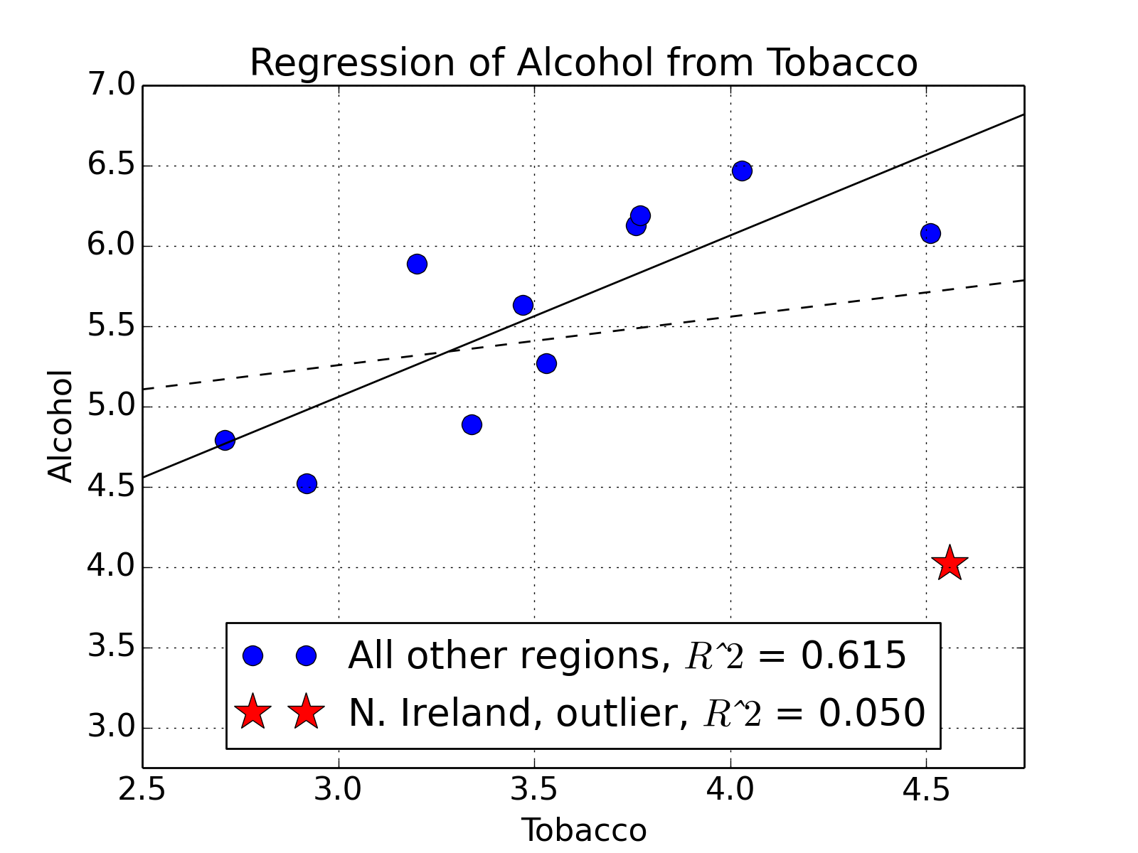
Comparison¶

Now that we have seen an example of linear regression with a reasonable degree of linearity, compare that with an example of one with a significant outlier. In practice, outliers should be understood before they are discarded, because they might turn out to be very important. They might signify a new trend, or some possibly catastrophic event.

X = df[['Tobacco','Eins']]
Y = df.Alcohol
result = sm.OLS( Y, X ).fit()
result.summary()

                            OLS Regression Results
==============================================================================
Dep. Variable:                Alcohol   R-squared:                       0.050
Model:                            OLS   Adj. R-squared:                 -0.056
Method:                 Least Squares   F-statistic:                    0.4735
Date:                Sun, 27 Apr 2014   Prob (F-statistic):              0.509
Time:                        12:58:27   Log-Likelihood:                -12.317
No. Observations:                  11   AIC:                             28.63
Df Residuals:                       9   BIC:                             29.43
Df Model:                           1
==============================================================================
                 coef    std err          t      P>|t|      [95.0% Conf. Int.]
------------------------------------------------------------------------------
Intercept      4.3512      1.607      2.708      0.024         0.717     7.986
Tobacco        0.3019      0.439      0.688      0.509        -0.691     1.295
==============================================================================
Omnibus:                        3.123   Durbin-Watson:                   1.655
Prob(Omnibus):                  0.210   Jarque-Bera (JB):                1.397
Skew:                          -0.873   Prob(JB):                        0.497
Kurtosis:                       3.022   Cond. No.                         25.5
==============================================================================

Regression Using Sklearn¶

*Scikit-learn (sklearn)* is an open source machine learning library for the Python programming language. It features various classification, regression and clustering algorithms.

In order to use sklearn, we need to input our data in the form of vertical vectors. Whenever one slices off a column from a NumPy array, NumPy stops worrying whether it is a vertical or horizontal vector. MATLAB works differently, as it is primarily concerned with matrix operations. NumPy, however has a matrix class for whenever the verticallness or horizontalness of an array is important. Therefore, in our case, we’ll cast the DataFrame as Numpy matrix so that vertical arrays stay vertical once they are sliced off the data set.

data = np.matrix( df )

Next, we create the regression objects, and fit the data to them. In this case, we’ll consider a clean set, which will fit a linear regression better, which consists of the data for all of the regions except Northern Ireland, and an original set consisting of the original data

cln = LinearRegression()
org = LinearRegression()

X, Y = data[:,2], data[:,1]
cln.fit( X[:-1], Y[:-1] )
org.fit( X, Y )

clean_score = '{0:.3f}'.format( cln.score( X[:-1], Y[:-1] ) )
original_score = '{0:.3f}'.format( org.score( X, Y ) )

The next piece of code produces a scatter plot of the regions, with all of the regions plotted as empty blue circles, except for Northern Ireland, which is depicted as a red star.

mpl.rcParams['font.size']=16

plt.plot( df.Tobacco[:-1], df.Alcohol[:-1], 'bo', markersize=10,
    label='All other regions, $Rˆ2$ = '+clean_score )

plt.hold(True)
plt.plot( df.Tobacco[-1:], df.Alcohol[-1:], 'r*', ms=20, lw=10,
    label='N. Ireland, outlier, $Rˆ2$ = '+original_score)

The next part generates a set of points from 2.5 to 4.85, and then predicts the response of those points using the linear regression object trained on the clean and original sets, respectively.

test = np.arange( 2.5, 4.85, 0.1 )
test = np.array( np.matrix( test ).T )

plot( test, cln.predict( test ), 'k' )
plot( test, org.predict( test ), 'k--' )

Finally, we limit and label the axes, add a title, overlay a grid, place the legend at the bottom, and then save the figure.

xlabel('Tobacco') ; xlim(2.5,4.75)
ylabel('Alcohol') ; ylim(2.75,7.0)
title('Regression of Alcohol from Tobacco')
grid()
legend(loc='lower center')

_images/alcohol_regressed_over_tobacco.png

Conclusion¶

Before you do anything, visualize your data. If your data is highly dimensional, then at least examine a few slices using boxplots. At the end of the day, use your own judgement about a model based on your knowledge of your domain. Statistical tests should guide your reasoning, but they shouldn’t dominate it. In most cases, your data will not align itself with the assumptions made by most of the available tests. Here is a very interesting article from Nature on classical hypothesis testing. A more intuitive approach to hypothesis testing is Bayesian analysis.

Assumptions¶

Standard linear regression models with standard estimation techniques make a number of assumptions about the predictor variables, the response variables and their relationship. Numerous extensions have been developed that allow each of these assumptions to be relaxed (i.e. reduced to a weaker form), and in some cases eliminated entirely. Some methods are general enough that they can relax multiple assumptions at once, and in other cases this can be achieved by combining different extensions. Generally these extensions make the estimation procedure more complex and time-consuming, and may also require more data in order to get an accurate model.

The following are the major assumptions made by standard linear regression models with standard estimation techniques (e.g. ordinary least squares):

Weak exogeneity. This essentially means that the predictor variables $x$ can be treated as fixed values, rather than random variables. This means, for example, that the predictor variables are assumed to be error-free, that is they are not contaminated with measurement errors. Although not realistic in many settings, dropping this assumption leads to significantly more difficult errors-in-variables models.
Linearity. This means that the mean of the response variable is a linear combination of the parameters (regression coefficients) and the predictor variables. Note that this assumption is much less restrictive than it may at first seem. Because the predictor variables are treated as fixed values (see above), linearity is really only a restriction on the parameters. The predictor variables themselves can be arbitrarily transformed, and in fact multiple copies of the same underlying predictor variable can be added, each one transformed differently. This trick is used, for example, in polynomial regression, which uses linear regression to fit the response variable as an arbitrary polynomial function (up to a given rank) of a predictor variable. This makes linear regression an extremely powerful inference method. In fact, models such as polynomial regression are often “too powerful”, in that they tend to overfit the data. As a result, some kind of regularization must typically be used to prevent unreasonable solutions coming out of the estimation process. Common examples are ridge regression and lasso regression. Bayesian linear regression can also be used, which by its nature is more or less immune to the problem of overfitting. (In fact, ridge regression and lasso regression can both be viewed as special cases of Bayesian linear regression, with particular types of prior distributions placed on the regression coefficients.)
Constant variance (aka homoscedasticity). This means that different response variables have the same variance in their errors, regardless of the values of the predictor variables. In practice this assumption is invalid (i.e. the errors are heteroscedastic) if the response variables can vary over a wide scale. In order to determine for heterogeneous error variance, or when a pattern of residuals violates model assumptions of homoscedasticity (error is equally variable around the ’best-fitting line’ for all points of x), it is prudent to look for a “fanning effect” between residual error and predicted values. This is to say there will be a systematic change in the absolute or squared residuals when plotted against the predicting outcome. Error will not be evenly distributed across the regression line. Heteroscedasticity will result in the averaging over of distinguishable variances around the points to get a single variance that is inaccurately representing all the variances of the line. In effect, residuals appear clustered and spread apart on their predicted plots for larger and smaller values for points along the linear regression line, and the mean squared error for the model will be wrong. Typically, for example, a response variable whose mean is large will have a greater variance than one whose mean is small. For example, a given person whose income is predicted to be $100,000 may easily have an actual income of $80,000 or $120,000 (a standard deviation]] of around $20,000), while another person with a predicted income of $10,000 is unlikely to have the same $20,000 standard deviation, which would imply their actual income would vary anywhere between -$10,000 and $30,000. (In fact, as this shows, in many cases – often the same cases where the assumption of normally distributed errors fails – the variance or standard deviation should be predicted to be proportional to the mean, rather than constant.) Simple linear regression estimation methods give less precise parameter estimates and misleading inferential quantities such as standard errors when substantial heteroscedasticity is present. However, various estimation techniques (e.g. weighted least squares and heteroscedasticity-consistent standard errors) can handle heteroscedasticity in a quite general way. Bayesian linear regression techniques can also be used when the variance is assumed to be a function of the mean. It is also possible in some cases to fix the problem by applying a transformation to the response variable (e.g. fit the logarithm of the response variable using a linear regression model, which implies that the response variable has a log-normal distribution rather than a normal distribution).
Independence of errors. This assumes that the errors of the response variables are uncorrelated with each other. (Actual statistical independence is a stronger condition than mere lack of correlation and is often not needed, although it can be exploited if it is known to hold.) Some methods (e.g. generalized least squares) are capable of handling correlated errors, although they typically require significantly more data unless some sort of regularization is used to bias the model towards assuming uncorrelated errors. Bayesian linear regression is a general way of handling this issue.
Lack of multicollinearity in the predictors. For standard least squares estimation methods, the design matrix $X$ must have full column rank $p$; otherwise, we have a condition known as multicollinearity in the predictor variables. This can be triggered by having two or more perfectly correlated predictor variables (e.g. if the same predictor variable is mistakenly given twice, either without transforming one of the copies or by transforming one of the copies linearly). It can also happen if there is too little data available compared to the number of parameters to be estimated (e.g. fewer data points than regression coefficients). In the case of multicollinearity, the parameter vector $\beta$ will be non-identifiable, it has no unique solution. At most we will be able to identify some of the parameters, i.e. narrow down its value to some linear subspace of $R^p$. Methods for fitting linear models with multicollinearity have been developed. Note that the more computationally expensive iterated algorithms for parameter estimation, such as those used in generalized linear models, do not suffer from this problem — and in fact it’s quite normal to when handling categorical data|categorically-valued predictors to introduce a separate indicator variable predictor for each possible category, which inevitably introduces multicollinearity.

Beyond these assumptions, several other statistical properties of the data strongly influence the performance of different estimation methods:

The statistical relationship between the error terms and the regressors plays an important role in determining whether an estimation procedure has desirable sampling properties such as being unbiased and consistent.
The arrangement, or probability distribution of the predictor variables $x$ has a major influence on the precision of estimates of $\beta$. Sampling and design of experiments are highly-developed subfields of statistics that provide guidance for collecting data in such a way to achieve a precise estimate of $\beta$.

Interpretation¶

A fitted linear regression model can be used to identify the relationship between a single predictor variable $x_j$ and the response variable $y$ when all the other predictor variables in the model are “held fixed”. Specifically, the interpretation of $\beta_j$ is the expected change in $y$ for a one-unit change in $x_j$ when the other covariates are held fixed—that is, the expected value of the partial derivative of $y$ with respect to $x_j$. This is sometimes called the ”unique effect” of $x_j$ on ”y”. In contrast, the ”marginal effect” of $x_j$ on $y$ can be assessed using a correlation coefficient or simple linear regression model relating $x_j$ to $y$; this effect is the total derivative of $y$ with respect to $x_j$.

Care must be taken when interpreting regression results, as some of the regressors may not allow for marginal changes (such as dummy variables, or the intercept term), while others cannot be held fixed (recall the example from the introduction: it would be impossible to “hold $t_j$ fixed” and at the same time change the value of $t_i^2$.

It is possible that the unique effect can be nearly zero even when the marginal effect is large. This may imply that some other covariate captures all the information in $x_j$, so that once that variable is in the model, there is no contribution of $x_j$ to the variation in $y$. Conversely, the unique effect of $x_j$ can be large while its marginal effect is nearly zero. This would happen if the other covariates explained a great deal of the variation of $y$, but they mainly explain variation in a way that is complementary to what is captured by $x_j$. In this case, including the other variables in the model reduces the part of the variability of $y$ that is unrelated to $x_j$, thereby strengthening the apparent relationship with $x_j$.

The meaning of the expression “held fixed” may depend on how the values of the predictor variables arise. If the experimenter directly sets the values of the predictor variables according to a study design, the comparisons of interest may literally correspond to comparisons among units whose predictor variables have been “held fixed” by the experimenter. Alternatively, the expression “held fixed” can refer to a selection that takes place in the context of data analysis. In this case, we “hold a variable fixed” by restricting our attention to the subsets of the data that happen to have a common value for the given predictor variable. This is the only interpretation of “held fixed” that can be used in an observational study.

The notion of a “unique effect” is appealing when studying a complex system where multiple interrelated components influence the response variable. In some cases, it can literally be interpreted as the causal effect of an intervention that is linked to the value of a predictor variable. However, it has been argued that in many cases multiple regression analysis fails to clarify the relationships between the predictor variables and the response variable when the predictors are correlated with each other and are not assigned following a study design.

101_modeling.ipynb

modeling.py

Bootstrapping¶

Another type of modelling is bootstrapping/. Sometimes you have data describing a distribution, but do not know what type of distribution it is. So what can you do if you want to find out e.g. confidence values for the mean?

The answer is bootstrapping. Bootstrapping is a scheme of resampling, i.e. taking additional samples repeatedly from the initial sample, to provide estimates of its variability. In a case where the distribution of the initial sample is unknown, bootstrapping is of especial help in that it provides information about the distribution.

102_bootstrap.ipynb

bootstrap.py

Table Of Contents

Previous topic

Next topic

This Page